Many students (and a few academics) erroneously see steam plant as "old" technology. In addition to conventional plant steam is used in combined cycle gas turbines to boost efficiency. Steam is employed in nuclear plant, geothermal plant and in solar plant. A cutting-edge topic is the production of work from "low grade" heat: this requires new working fluids with features not dissimilar to those of steam. A study of vapour compression heat pumps benefits from the insights offered by steam plant.
These notes are comparable to four lectures delivered to a Year 2 Mechanical Engineering class. It was my intention that students should be able to:
Identify the unit operations in basic steam cycles.
Identify the key features of individual cycles.
Present the cycles in the form of plant diagrams and TS diagrams.
Carry out energy balances on the individual unit operations, and thereby calculate cycle performance parameters.
We have presented the properties of air which - for engineering purposes - behaves as an ideal gas and follows simple laws. Steam rarely behaves as an ideal gas and to obtain its properties one resorts to computer programmes, charts or tables. Moreover, in practically all thermodynamic cycles steam undergoes a change of phase . It is converted from liquid to vapour in a boiler and from vapour to liquid in a condenser.
Notes on the properties of steam and water are
available here . There is also an
interactive Ts chart . Let us recall key features of working with steam (steam isobars are shown on Figure 1 - a Ts chart).
The pressure increases (almost) exponentially with temperature.
In a boiler, equilibrium is achieved between a large mass of liquid and a comparatively small mass of vapour. There is always conversion of vapour molecules to liquid and liquid molecules to vapour. At equilibrium these conversions are equal.
If the vapour mass is infinitesimally small the liquid is said to be saturated. Conversely if the liquid mass is infinitesimally small the vapour is said to be saturated.
For a given temperature there is a single saturation pressure, \(p_{sat}(T)\) and for a given pressure there is a single saturation temperature, \(T_{sat}(p)\)
On the vapour-liquid curve there is just one degree of freedom. That is, all thermodynamic properties can be estimated if just one property (T, p, s, h) is known.
When heated above its saturation temperature steam is termed "superheated steam" (to the right of the water-vapour curve).
When cooled below its saturation temperature water is termed "subcooled water" (to the left of the water-vapour curve).
The end points are the triple point and the critical point (students may want to investigate further on the internet or in the course text).
Figure 1 Ts diagram for water. Isobars (curves of constant pressure) are labelled with their corresponding pressure. The red curve labelled 'f' represents saturated liquid whereas the blue curve labelled 'g' represents saturated vapour.
3. Steam Plant Components
In simple steam plant components, either heat is transferred or
work is transferred.
Starting with liquid water at typically 30\(^oC\) and 42 mbar the following operations happen cyclically in a steam plant:
the water is pressurised (say to 20 bar);
it is heated and boils to form steam;
it is expanded and drives a turbine, producing power and returning the exhaust to the original pressure (here about 42 mbar);
it is condensed.
For a proposed design of power plant one wants to predict several performance parameters and in particular cycle efficiency. Cycle efficiency is the useful work derived per unit of heat input to the boiler (it excludes heat losses in the combustion chamber). We shall describe here, one by one, the components in the simple Rankine cycle. The protocol is: operation of plant; thermodynamic path (TS diagram); energy balance.
The feedwater pump takes in water at the condenser pressure and produces water at the boiler pressure. Heat addition in the boiler converts sub-cooled water to saturated steam.
Let us start with saturated liquid - feedwater - at very low pressure (about 40 mbar) and close to room temperature (about 20 \(^oC\)). In conformity with
Rogers and Mayhew
this stream of fluid is Stream 4. It is required to convert this to saturated vapour at higher pressure (typically 20 bar).
Operation of plant (see Figure 2) - the feedwater pump (A) uses a comparatively small amount of power to pressurise water to its target pressure (at stream 5). Displacement work is needed (to force fluid past boundaries) but water is practically incompressible and practically no work of compression is done. Pressurised water then passes to the feedwater drum (B, part of the boiler). A thermosyphon effect causes fluid to rise to the steam drum (C) via generator tubes (F)- wherein it partially boils forming wet steam. The steam drum separates liquid and saturated vapour. Saturated vapour (stream 2) then passes to the turbine.
Later in this section (as per many text books) we shall represent the entire boiler (parts B,C,D,E and contained within control surface C.S.2) with a single block on a block diagram.
Figure 2 Parts of the Rankine cycle - Feedwater pump (A) and boiler. The boiler comprises feedwater drum (B), steam drum (C), generating tubes (F) and downcomers (E).
Thermodynamic path - the feedwater pump (streams 4 to 5) pressurises liquid water with a large change in pressure but minimal change in other properties (T, s, h). (If you were to generate a Ts diagram with a computer programme you would have to zoom in on this feature to make it visible.) The pressurised water in stream 5 is colder than its new saturation temperature ( \(212^oC\) on Figure 2 ) and is hence sub-cooled. The Ts diagram on Figure 3 shows boiler operation as paths 5-to-1-to-2. The paths lies on an isobar along which the pressure is a constant 20 bar.
Path 5-to-1 represents the complex heating processes changing sub-cooled water to saturated. Path 1-to-2 represents boiling.
Energy balance - two rates of energy flow are needed. Consider merging controls surfaces C.S.1. and C.S. 2 to cut streams 5 and 2 (Figure 2). Then the mechanical power supplied to the pump and the boiler heating power are
\begin{equation}
\dot{W}_{45} + \dot{Q}_{52} = \dot{m}_{steam}(h_2 - h_4)
\end{equation}
It is sometimes appropriate to write the balance in terms of specific work and specific heat (that is, energy per unit mass),
Assumptions include: no substantial change in potential or kinetic energy; no unwanted heat loss in transport pipes; steady conditions.
At 2 vapour is saturated and \(h_2 = h_g(p_2)\) can be found in tables. At 4 liquid is saturated and \(h_4=h_f(p_4)\) can also be found in tables.
The enthalpies should be easily found by clicking on the appropriate points on our online Ts diagram (or use the "number input(p,T,x)" button).
Given that the feedwater is practically incompressible, pressurisation causes no change in internal energy or temperature and no change in specific volume (\(v_2=v_4=v\)). Consider on Figure 2 control surface C.S.1 which cuts streams 4 and 5.
If one considers shaft work in open systems
(see final part of linked section 4)
\begin{equation}
w_{45} = \int_1^2 v dp \approx \frac{p_5-p_4}{\rho_f}
\end{equation}
where \(\rho_f\) is the enthalpy of liquid water. Not all tables include the density of water and an estimate of \(1000 kg m^{-3} \) is often used. The corresponding inaccuracy for a boiler pressure of 30 bar would be in the region of 10% of feedwater pump work and a very small proportion of net work (see below). Take care, however, with modern plant where feedwater pressure is raised well above the critical pressure of 221 bar. The values of \(h_2, h_4, p_4, p_5 \) yield sufficient information to calculate the specific heat input to the plant, \(q_{52}\).
Figure 3 Ts diagram of incomplete Rankine cycle (Figure 2) showing (4-to-5) pressurisation from condenser to boiler pressure, (5-to-1) heating to the boiler pressure; at point 1 we find saturated liquid, (1-to-2) further heating in the boiler, transforming saturated liquid to saturated vapour.
Example 6B.010: heat supplied to the boiler. Find the heating rate in the boiler shown on Figure 2
(Take a steam flow rate of 50 kg/s and otherwise use the values, assumptions, nomenclature and diagrams from this section.)
Solution: See Figures 2 and 3 above.Stream 4 is saturated water at 20 \(^oC\) such that \(h_4 = 84 kJ \, kg^{-1}\) and \(p_4 = 0.02337 bar\) . Stream 2 is saturated vapour at 20 bar such that \(h_2 = 2799 kJ \, kg^{-1}\) . Then from SFEE
\begin{equation*}
\dot{W}_{45} + \dot{Q}_{52} = 50 \times (2799-84) = 135 \; 750 kW
\end{equation*}
From the equation for pump work
\begin{align*}
\dot{W}_{45} &= \frac{\dot{m}_{steam}(p_5-p_4) }{\rho}\\
& = 50 kg \,s^{-1} (20 - 0.02337) bar \times [100 kN \, m^{-2} \, bar^{-1}]/1000 kg \,m^{-3} = 100 kW
\end{align*}
$$ \dot{Q}_{52} = 135 \; 750 -100 = 135 \; 650 \; kW $$
Note that in the main text I stated that my estimate of work for the boiler feedwater pump (with 30 bar pressure achieved) might be subject to inaccuracies of 10 per cent, or in this case 10 kW. This is a very small proportion of overall work.
Turbine
The turbine generates power. Steam leaves the turbine at condenser pressure.
Operation of plant, Figure 4 -the turbine is a single item of plant (although we shall see elsewhere that it contains several stages). In the Rankine cycle saturated steam enters and wet steam exits. In practice this is problematic because liquid droplets will erode rotor blades.
Thermodynamic path - saturated stream enters the turbine at stream 2 and wet steam exits at stream 3. The reduction in enthalpy corresponds to work output. A reversible turbine operates isentropically - that is with constant entropy and \(s_3 \equiv s_{3,isen} = s_2\). If the turbine operates irreversibly \(s_3 > s_{3,isen} \) (but still \(s_{3,isen}= s_2\)) and we must know the
turbine's isentropic efficiency. In either instance erosion means that we should compute outlet steam quality in addition to mechanical power. On the Ts diagram, Figure 5, we draw attention to the low pressure isobar on which lies the states of the turbine exit (at 3 and 3isen), saturated liquid (f) and saturated vapour (g).
Energy balance - we ignore heat loss from the turbine, assume steady conditions, and ignore changes in potential and kinetic energy.
\begin{align*}
\dot{W}_{23} &= \dot{m}_{steam} (h_3-h_2) \qquad or \qquad w_{23}=h_3-h_2\\
\dot{W}_{isen,23} &= \dot{m}_{steam} (h_{3,isen}-h_2) \qquad or \qquad w_{isen,23}=h_{3,isen}-h_2
\end{align*}
The subscript \(_{isen}\) indicates the special reversible, isentropic case (as does ' on Figure 5 - I shall change this in time). Here entropy is unchanged, \(s_{isen,3}=s_2 \). For the
interactive, graphical solution plot a vertical isentropic line through 2, to intersect the low pressure isobar at 3,isen. (Then click on this point to get the dryness fraction and enthalpy). For "pen and paper" calculations \(s_{isen,3}\) can be related to the two saturation entropies (at low pressure) to yield steam quality. By adapting the "wet property" equation, one gets from three known entropies,
\begin{equation*}
s_{isen,3} = s_2 = (1-x_{isen,3}) s_f + x_{isen,3} s_g \implies x_{isen,3}
\end{equation*}
(Remember that the values of saturation entropies \(s_f\) and \(s_g\) should be found at the turbine exit pressure, \(p_3\)). The enthalpy follows from known dryness fraction and saturation enthalpies,
\begin{equation*}
h_{3,isen} = (1-x_{3,isen}) h_f + x_{3,isen} h_g
\end{equation*}
(Like the saturation entropies, the saturation enthalpies should also be found at \(p_3\)). An irreversible turbine is characterised by an isentropic efficiency (found by measurement).
$$ \dot{W}_{23} = \eta_{isen} \dot{W}_{isen,23} \qquad or \qquad w_{23} = \eta_{isen} w_{isen,23} $$
An anisentropic and irreversible expansion merits an updated estimate of dryness fraction. The new exit enthalpy, \(h_3\), can be computed from SFEE; this, plus the saturation enthalpies, implies the updated dryness fraction.
\begin{align*}
h_3 =& h_2+w_{23} \\
h_3=& (1-x_3) h_f(p_3) + x_3 h_g (p_3) \implies x_3
\end{align*}
Figure 4 Symbol for turbine. Positions 2 and 3 refer to the Rankine cycle such that the inlet is saturated vapour and the exit is wet steam (a) representative version (b) symbol.
Figure 5 Ts diagrams for turbine expansion showing reversible and irreversible paths (2 to 3' and 2 to 3, using ' to indicate isentropic here). Note that the low pressure isobar takes in turbine exit condition and conditions of saturated liquid (f) and saturated vapour (g). The dotted line shows the previous action of the feedwater pump and boiler.
Example 6B.020: turbine power. Consider the saturated steam developed by a boiler operating at 20 bar (see last lecture). This is to fed to a turbine. Find the power from the turbine for (1) reversible operation (2) an isentropic efficiency of 85%.
(Take the outlet pressure as \(p_3 =0.02337 \, bar\) and otherwise use the values, assumptions, nomenclature and diagrams from this section.)
Solution: Stream 2 is saturated vapour at 20 bar such that \(h_2 = 2799 \, kJ \, kg^{-1}\) and \(s_2= 6.340 \, kJ \, kg^{-1} \,K^{-1}\). Stream 3 corresponds to a saturation temperature \(T_3 = 20^oC\) and other corresponding properties (at the lower pressure) are \(s_f = 0.296\, kJ \, kg^{-1} \, K^{-1}, s_g = 8.666\, kJ \, kg^{-1} \, K^{-1}, h_f = 84 \,kJ\,kg^{-1}, h_g = 2538 \, kJ \, kg^{-1}\). Apply the wet property equation,
\begin{align*}
s_{isen,3}=s_2= 6.340 &= (1-x_{isen,3}) \times 0.296 + x_{isen,3} \times 8.666 \implies
x_{isen,3} = 0.722 \\
h_{isen,3} &= (1-0.722) \times 84 + 0.722 \times 2538 = 1856 kJ \, kg^{-1}
\end{align*}
From the SFEE,
\begin{align*}
\dot{W}_{isen,23} = \dot{m}_{steam} (h_{isen,3}-h_2) = 50 \times (1856-2799) = -47 \,150 kW \\
\dot{W}_{23} = \eta_{isen} \dot{W}_{isen,23} = 0.85 \times (-47 \,150) = -40 \,078 kW
\end{align*}
Condenser
Low pressure steam rejects heat and condenses.
Figure 6 shows the plant diagram for the complete Rankine cycle and in particular the location of the condenser. The condenser converts low pressure steam to liquid - the steam must reject heat to the condenser's coolant.
Operation of Plant - The condenser lies between the turbine outlet and the feedwater pump inlet, and therefore has inlet stream 3 and outlet stream 4. It will be assumed that the condenser operates isobarically (that is, that friction effects are too small to change pressure appreciably), that is \(p_3=p_4\). In the current example the steam at inlet is wet steam and we assume that saturated liquid exits the condenser. We have found already enthalpies \(h_3, h_4\) and the heat output from the condenser follows from SFEE.
Energy Balance - In principle we have already calculated all heat inputs and all work output to enable calculation of cycle efficiency. However, it is good practice to check that estimates conform to the first law (that is, all net energy inputs (heat and work) sum to zero). The SFEE can be applied to the condenser
\begin{equation*}
\dot{Q}_{34} = \dot{m}_{steam} (h_4-h_3) \qquad or \qquad q_{34} = h_4-h_3
\end{equation*}
Example 6B.030:heat rejected from a condenser. Find the heat rejection from a condenser operating at a saturation temperature of 20\(^oC\) and accepting steam from the turbine described in Example 6B.020. Assume that the expansion was isentropic.
Solution: The previous example provided an estimate of \(h_3\) (isentropic version), vis \( h_{isen,3} = 1856 kJ \, kg^{-1} \).
Saturated liquid is assumed to exit the condenser at \(T_4=20^oC\) so that \(h_4 = h_f = 84 kJ kg^{-1}\). From the SFEE,
\begin{align*}
\dot{Q}_{34} = \dot{m}_{steam} (h_4-h_3) = 50 \times (84-1856) = -88 \,600 kW \\
\end{align*}
4. The Rankine Cycle
The calculations thus far are summarised. Refer to the plant diagram (Figure 6) and the Ts diagram (Figure 7).
We start with the condensate which is delivered to the inlet of the feedwater pump, stream 4. The feedwater pump demands a comparatively small power input and any changes in entropy or temperature are small. The water in stream 5 has been pressurised. The feed pump work is comparatively small.
$$ w_{45} \approx \frac{p_5-p_4}{\rho} \qquad feed \; pump \; work \; (per \; kg) $$
We assume isobaric operation of the boiler so that \(p_5=p_1=p_2\). Water changes from subcooled liquid (at 5) to saturated liquid (at 1) to saturated vapour (at 2). Heat is added in the boiler ( from 5-to-1-to-2).
Saturation properties at 4 and 2 can be found easily from steam tables, charts or computer programs. The feed pump requires a comparatively small amount of specific work to pressurise water; consequently the enthalpy \(h_5\) is slightly more than \(h_4\). For a control surface cutting streams 4 and 2, the SFEE yields the heat input to the boiler, \(q_{52}\).
In the first instance we assume isentropic (constant entropy) operation of the turbine. The
wet property relationships
relate three entropies at low pressure (turbine exit (3), saturated liquid (f), saturated vapour (g)) to the steam quality and hence wet steam enthalpy \(h_{isen,3}\) (see Example 6B.020 above). Application of the SFEE between streams 2 and 3 yields turbine work,
$$ w_{isen,23} = h_{isen,3}-h_2 \qquad \; isentropic \; work \; (per \; kg) $$
An isentropic efficiency is employed to get the power from a real world turbine.
Work ratio is the ratio of net work to turbine work. Net work = turbine work - feedwater pump work. This is very close to 100% whereas for a Brayton cycle it is closer to 70%. The higher work ratio tends towards a smaller turbine size for a given power output and thus a lower capital cost of plant.
Specific steam consumption (SSC) is the reciprocal of work per unit mass of steam (w). It is usually quoted in kW hr/kg (note 1 kW hr = 3 600 kJ). A lower SSC facilitates smaller transport pipes and lower costs of plant construction. (The minimum pipe diameter is calculated to keep pressure losses reasonably small.)
Cycle efficiency is the ratio of net power output to heat input. Note that net work is turbine work - feedwater pump work (although it is sometimes acceptable to neglect FWP terms).
Isentropic efficiency is an attribute of the turbine rather than the plant. It is the ratio of real turbine power to turbine power under reversible conditions (for the same start and end pressures).
Figure 6 Plant diagram for a Rankine Cycle.
Figure 7 Ts diagrams for complete Rankine cycle.
Useful indicators (above) include the cycle efficiency , the ratio of net power output to heat input (to the cycle). This is a little different to plant efficiency, because plant efficiency allows for heat losses from the boiler. In terms of an equation.
Recall that here heat input is via the boiler only; do not include the condenser. (The work terms include the turbine and feedwater pump. One might argue that there is only one heat input (from 5-to-2-to-1) but in the reheat cycle (next lecture) two or more distinct heat additions are evident.)
Example 6B.040: Cycle Efficiency - Restarting most previous calculations, find the cycle efficiency for a Rankine cycle operating between pressures of 0.02377 bar (saturation temperature \(20^oC\)) and 20 bar. Assume isentropic expansion of steam
and take the feed pump work as \(2 kJ kg^{-1} \).
Solution:
Draw the isobars at 0.02337 bar (saturation temperature \(20^oC\)) and 20 bar).
Figure 40A Construction of isobars at boiler pressure (20 bar) and condenser pressure (0.02337 bar)
Find properties at 4(saturated liquid at 0.02337 bar) and 2 (saturated vapour at 20 bar). Using the online tool,
(The "point and click" facility is vulnerable to manual error, particularly for saturated liquid. I believe it is adequate for many educational purposes. Better accuracy follows from steam tables, or from the online plotters "number input (p,T,x) button". )
Draw a control surface (CS) cutting streams 2 and 4
Draw a vertical isobar through point 2. Mark as "3" the point of intersection with the lower pressure
isobar (p=0.02337bar)
Figure 40B Vertical isentropic line indicates operation of turbine from 2 to 3
From the online tool note the enthalpy and dryness fraction at 3
$$h_3 = 1862 kJ kg^{-1} \qquad x_2 = 72.4\% $$
(Confirm, by reading values of the online tool, that the horizontal length from point 3 to the saturated liquid curve (6.3-0.3=6 approx.) is roughly
72% of the length from the saturated liquid curve to the saturated vapour curve (8.7-0.3=8.4 approx).)
The work ratio for a Rankine cycle is close to 100 per cent.
$$ work \; ratio = \frac{w_{tot}}{w_{23}}=\frac{-934}{-936} = 99.8\% $$
Finally, mark up the remaining points 1 and 5 on the screen dump, and mark up the cycle.
Figure 40C Mark up of cycle
5. Rankine Cycle with Superheat
A superheater advantageously raises the temperature of steam above its saturation temperature.
There are a number of ways of increasing cycle efficiency, including superheat, reheat, regenerative heating and an economiser.
To obtain a good efficiency, we need as high a temperature as possible at the turbine inlet. The exponential increase of saturation pressure with respect to temperature can create problematic mechanical stresses in the boiler. (In the 19th century,
boiler explosions were not unknown.) To obtain good cycle efficiency at reasonable working pressure, saturated steam is heated above its saturation temperature; the steam is then said to be "superheated". To achieve the superheat condition steam flows from the boiler tubes, to a separate bank of tubes within the combustion chamber. This superheater thereby increases steam temperature but not steam pressure. A further advantage of superheating is that elsewhere in the cycle wet steam emerges from the turbine with a more acceptable dryness fraction. A dryness fraction less than 90% is generally recommended for axial turbines, to prevent unacceptable erosion. Figure 8 shows the plant diagram and Figure 9 shows the Ts diagram. (The numbering convention of
Rogers and Mayhew
is followed.) The cycle is as follows:
streams 1-2: The feedwater pressure is raised from very low (less than 0.1 bar) to high (maybe 30 bar);
streams 2-3-4: The boiler changes the state of fluid from saturated liquid to saturated vapour;
streams 4-5: Steam is further heated isobarically so that it is superheated. (Note - I have shown the boiler as a single block here, as opposed to the more detailed view in Figure 2);
streams 5-6: The turbine expands steam (isentropically in Figure 9) and power is produced;
streams 6-1: The turbine exhaust is condensed.
Figure 8: Plant diagram for a Rankine Cycle with superheat. A set of tubes - the superheater (streams 4 to 5) - is taken back into the combustion chamber and steam temperature is raised above the saturation value. (Note that stream 1 is now the condenser exit, in conformity with Rogers and Mayhew)
Figure 9 Ts diagram for superheat cycle. Note that point 5 is distant from the saturation curve (g)
Example 6B.050: Superheat cycle. In a Rankine cycle with superheat, condensate exits the condenser at 25\(^oC\) and the boiler operates at 30 bar. The superheater further raises the steam temperature to 400 \(^oC\) (but still at 30 bar). You should ignore the power supplied to the feedwater pump. The turbine acts isentropically. (a) Find the cycle efficiency. (b) Find the cycle efficiency if the isentropic efficiency of the turbine is 85%.
Solution: I used my online plotter.
Draw isobars corresponding to 0.03166 bar (saturation temperature \(=25^oC\) ) and 30 bar. On the 0.03166 bar isobar, mark as point 1 the condenser exit and on the 30 bar isobar mark as point 5 the superheater exit.
Figure 50A Construction of isobars at boiler pressure (30 bar) and condenser pressure (0.03166 bar). The condenser exit
is marked as 1 and the superheater exit is marked as 5
Draw a vertical line of constant entropy through point 5, representing expansion in the turbine. Label as point 6 the intersection between this isentropic line and the low pressure isobar (for p = 0.03166 bar). Then read the enthalpy and dryness fraction at this point.
Figure 50B Isentropic expansion in turbine, from 5 to 6
$$ h_6=2060 kJ kg^{-1} \qquad x_6 = 0.801 $$
(Sanity check, reading data from the online plotter "by eye": \( x_6 \approx (6.9-.4)/(8.6-.4) \approx 79\% \) ✓ .)
Apply SFEE to get total input (CS from 1-to-5) and isentropic turbine work (CS from 5-to-6)
\begin{align*}
q_{51} &= h_5-h_1-w_{12} \approx h_5-h_1 \approx 3231-104 \approx 3127 \; kJ kg^{-1} \qquad total \; heat \; input \\
w_{tot} \approx w_{isen,56} &= h_6-h_5 = 2060-3231 = -1,171 \; kJ kg^{-1} \qquad \; total \; work \;(ignore \; feed \; pump) \\
\eta_{cyc} &= \frac{|w_{tot}| }{q_{51}} \approx
\frac{1171}{3127}=37.4\% \qquad cycle \; efficiency \;
\end{align*}
This is 3% greater than the simple Rankine cycle.
(The feed pump work is 3kJ/ kg. This could be substructed from both the numerator and denominator of cycle efficiency. The (slight) improvement in accuracy is evident only in the fourth significant figure).
For part (b) the heat input \(q_{15}\) remains the same and feed pump work is ignored. Allow for isentropic efficiency to get a new work output and hence a newcycle efficiency.
The dryness fraction is increased. (A sanity check, by eye, for figure 50B gives the dryness fraction as
\(x_6 \approx (s_6-s_f)/(s_g-s_f) \approx (7.5-0.4)/(8.6-0.4) \approx 0.866 \) ✔
Example 6B.060: Saturated vapour at turbine outlet. The preceding cycle in Example 6B.050 is constructed with a turbine that operates irreversibly, and by happy coincidence saturated steam is evident at the turbine exhaust. Estimate the cycle efficiency and the isentropic efficiency of the turbine. (In 6B.050 condensate exits the condenser at 25\(^oC\) and the boiler operates at 30 bar. The superheater raises the steam temperature to 400 \(^oC\) (but still at 30 bar). You should ignore the power supplied to the feedwater pump.
Solution:
Figure 60A Irreversible expansion in turbine, from 5 to 6
The thermodynamic states at 1,2,3,4,5 are identical to those in the previous Example 6B.050. The only enthalpy to alter is the turbine exhaust enthalpy at point 6. At \( T_{sat}=25^oC, h_6 \equiv h_g = 2547 \, kJ \, kg^{-1}\). Thus the net work and turbine work are:
So long as feedwater pump work is neglected, the heat addition is not too different from the previous case and turbine power approximates to net power. The cycle efficiency approximates to,
Steam emerges from a first (HP) turbine at intermediate pressure rather than low pressure. Following reheat the steam passes to a second (LP) turbine.
In the reheat cycle roughly half the steam enthalpy is converted to work at high pressure, thereafter exhaust steam is led back to a reheater, and then a low pressure turbine. This results in both an increase in cycle efficiency and drier steam. Figure 10 shows the plant diagram and Figure 11 shows the TS diagram. The relevant points are as follows.
In stream 4, saturated steam exits the boiler.
In streams 4-5, steam is heated isobarically yielding superheated steam.
In streams 5-6, steam is expanded in the high pressure turbine.
In streams 6-7, steam at intermediate pressure is reheated.
In streams 7-8, steam is expanded in the low pressure turbine.
Figure 10 Plant diagram for superheat and reheat. A third heat exchanger acts on exhaust steam from the HP turbine - this reheated steam passes to the LP turbine
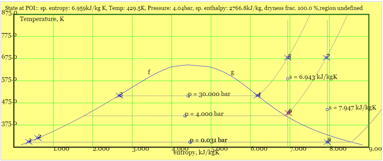
Figure 11 Ts diagram for Rankine cycle with superheat and reheat
Example 6B.070: Reheat cycle. In a reheat cycle, condensate exits the condenser at 25\(^oC\) and the boiler operates at 30 bar. A superheater further raises the steam temperature to 400 \(^oC\). The high pressure turbine acts reversibly and steam exits at 4 bar. The exhaust is reheated to 400 \(^oC\) and is again expanded isentropically. Estimate the cycle efficiency. (Ignore the power supplied to the feedwater pump.)
Solution: The Ts diagram is sketched below. Note that points 1,2,3,4,5 and corresponding energy flows were
evaluated in the previous Example 6B.060
Figure 70A Irreversible expansion in turbine, from 5 to 6
The cycle efficiency is then the ratio of work output to heat input.
$$\eta_{cycle} =\frac{|w_{tot}|}{q_{tot}} = \frac{1402}{3651} = 38.4 \% $$
For the isentropic expansions, this efficiency is 1% greater than for the superheat cycle and 4% greater than for the simple Rankine cycle.
7. Regenerative Cycles
Regenerative Cycles improve cycle efficiency by increasing the average temperature at which the working fluid accepts heat.
Vapour bled from an intermediate point in the turbine adds heat to the feedwater. There are two heating methods - open and closed feedwater heaters. In the open feedwater heater some steam is bled from the turbine and mixed with the feedwater to raise its temperature. By this means heat recovery inside the plant replaces some external heating.
Figure 11 Plant diagram for regenerative cycle with open feedwater heater
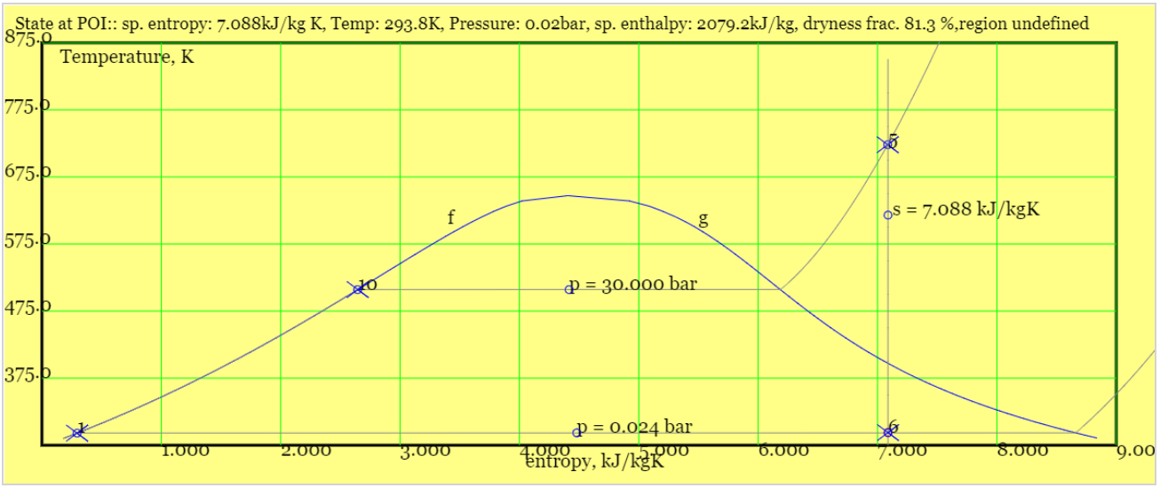
Figure 12 Ts diagram for regnerative cycle with open feedwater heater. Feedwater pump work is ignored so
points 2 and 4 are omitted. Point 10 is added as an extra point within the boiler.
The cycle processes associated with the open feedwater heater are listed below.
The condensate pressure is raised from low to intermediate (1-2).
Mixing of the feedwater (2) with bleed steam (7) produces hotter liquid at its saturation temperature (3).
Saturated liquid is pressurised further to the full boiler pressure (3-4).
Heat is transferred in the boiler and, if fitted, the superheater (4-5).
The turbine converts vapour enthalpy to work (5-6).
A fraction y of the vapour is bled(7) and passed to the open feedwater heater.
A large set of assumptions applies. As for other steam cycles, I shall assume steady conditions. I shall ignore losses of pressure in the boiler, condenser, feedwater heater and pipework. Changes in kinetic and potential energy will be ignored. Additional assumptions will be explained in the context of a worked example.
Example 6B.080: Regenerative cycle - Find the cycle efficiency for a regenerative cycle operating between pressures of 0.02377 bar (saturation temperature \(20^oC\)) and 30 bar. Assume (1) superheat to \(450^oC\) (2) the turbine operates reversibly and isentropically.
Solution:
Low and High Pressure Operation Operation
Plot online isobars for low pressure (0.02377bar) and high pressure (30bar). Mark locations of low pressure condensate (1), superheated steam (5), turbine outlet/ condenser inlet (6) and the point in the boiler where high pressure water is saturated (10). Plot a vertical line of constant entropy through the point 5 for superheated steam (this represents expansion in the turbine).
Figure 80A Low and high pressure isobars. Locations of saturated liquid (1,10) superheater outlet (4)
and turbine exhaust are marked.
From the online plotter
$$h_2 \approx h_1=83 kJ kg^{-1} \qquad h_{10}=h_f(30bar)=1008 kJ kg^{-1} \qquad T_{10}=507K = 314^oC$$
(
Weir
reports maximimum cycle efficiency for equal differences in liquid enthalpy. Temperature is easier to work with, and incurs only small deviations from the optimum.)
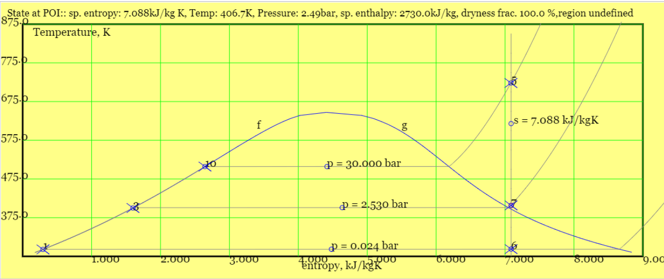
Mark point 3 on the Ts diagram and draw an isobar through it (p=2.5 bar). Mark the bleed point (7) where the
isobar of intermediate pressure intersects the vertical line of constant entropy.
In the closed feedwater heater the bleed steam surrenders its energy by heat transfer rather than mixing. The cycle thereby requires only one feedwater pump.
Figure 13 Plant diagram for regenerative cycle with closed feedwater heater
The complete cycle for the closed feedwater heater is listed below. I write differences with the open feedwater counterpart in italic font.
The condensate pressure is raised from low pressure to high, boiler pressure (1-2).
Heat transferred in the feedwater heater from the bleed stream (7) raises the feedwater
temperature (2-3).
Stream 4 is added to align stream numbers with the previous plant diagram. There is no process from (3-4) .
Heat is transferred in the boiler and, if fitted, the superheater (4-5).
The turbine converts vapour enthalpy to work (5-6).
A fraction y of the vapour is bled (7)and passed to the closed feedwater heater.
The vapour bleed condenses; heat then transfers to the feedwater heater .
Condensate is throttled and passed to the condenser (8-9).
The heat balance around the closed feedwater heater includes four streams rather than three (streams 1,9,3,7).
For isenthalpic expansion it is reasonable to expect \(h_8=h_9\) and given the weak effect of pressure on enthalpy \(T_8 \approx T_9\). If pump work
is neglected \(h_2 \approx h_1\). If heat transfer were to be highly effective such that \(T_8=T_2\ \implies T_9=T_1 \) then the heat balance would become practically the same as the open heater version. It is more likely that
\(T_8-T_1>0\); there is then an appreciable "terminal temperature difference">
The above example is purely illustrative. Typical industrial plant designs would
allow for eight or nine feedwater heaters, perhaps with one (and one only) operating as open so
as to de-aerate steam (air impedes condensation and contributes to corrosion).
A train of closed heaters reduces the number of pumps required. Regeneration would operate typically with superheat and double reheat. Wales et al.
offer a literature search and adjusted plant diagram.

 Figure 1 Ts diagram for water. Isobars (curves of constant pressure) are labelled with their corresponding pressure. The red curve labelled 'f' represents saturated liquid whereas the blue curve labelled 'g' represents saturated vapour.


 Figure 40A Construction of isobars at boiler pressure (20 bar) and condenser pressure (0.02337 bar)
 Figure 40B Vertical isentropic line indicates operation of turbine from 2 to 3
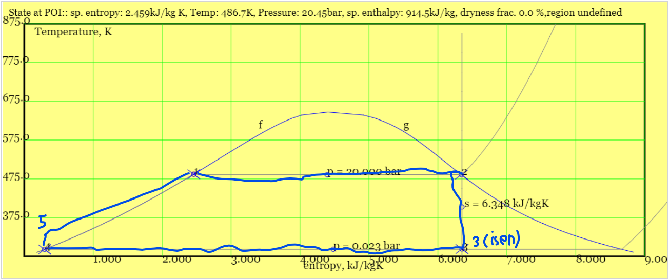 Figure 40C Mark up of cycle


 Figure 50A Construction of isobars at boiler pressure (30 bar) and condenser pressure (0.03166 bar). The condenser exit
is marked as 1 and the superheater exit is marked as 5
Figure 50A Construction of isobars at boiler pressure (30 bar) and condenser pressure (0.03166 bar). The condenser exit
is marked as 1 and the superheater exit is marked as 5
 Figure 50B Isentropic expansion in turbine, from 5 to 6
$$ h_6=2060 kJ kg^{-1} \qquad x_6 = 0.801 $$
Figure 50B Isentropic expansion in turbine, from 5 to 6
$$ h_6=2060 kJ kg^{-1} \qquad x_6 = 0.801 $$
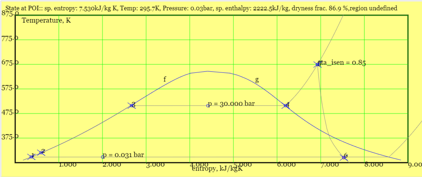 Figure 50C Irreversible expansion in turbine, from 5 to 6.
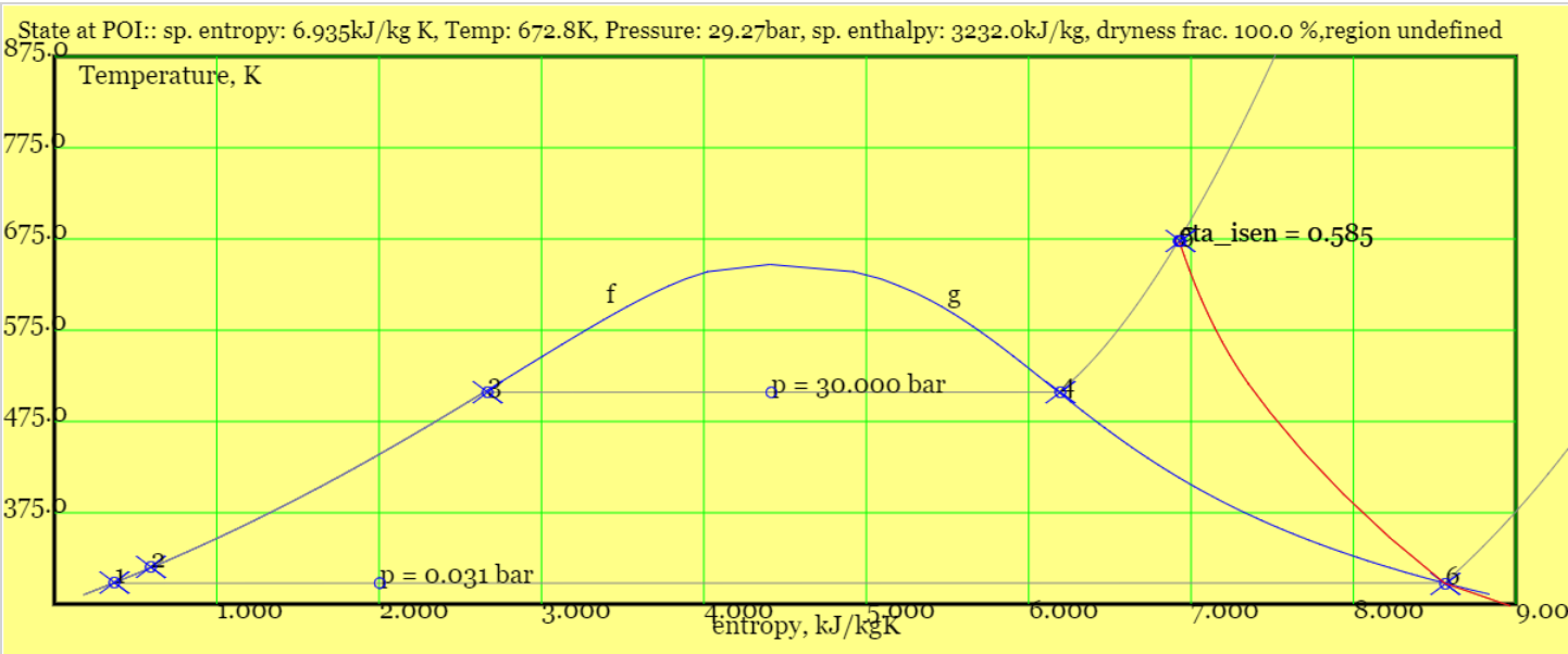 Figure 60A Irreversible expansion in turbine, from 5 to 6