Mass crosses the boundaries of an open system and thereby transports energy.
Up to now we have looked at non-flow processes occurring in closed systems, that is to say systems within which the working fluid is effectively "trapped" within a container so that its mass remains unchanged. Very few processes in engineering are like this, however. The vast majority consist of flow processes, in which a working fluid is continually passing into, and out of, a system. The fluid will probably undergo some change in the process, either in temperature or pressure or even chemical composition. Most of these processes are continuous, that is to say fluid properties do no vary significantly
with time, and we can refer to processes of this nature as steady flow processes. This does not rule out from this analysis such things as reciprocating internal combustion engines or reciprocating compressors, provided that the period over which we average our various mass flows is large compared to the period of the individual cycles. The reciprocating internal combustion engine operates (arguably) as a rapidly series of identical non-flow processes, but if we restrict our attention to the time-averaged flows of, say, the air, fuel, cooling water and exhaust, we shall be able to analyse it as a steady flow system. The steady flow analysis cannot be applied with any accuracy where changes in operating condition are taking place, particularly if they are fairly rapid. The starting, stopping and warming parts of a plant demands more detailed analysis than that given by the steady flow approach – but for most plant the first design activity covers operation under normal, steady load, conditions.
2.) Mass Conservation
The cross section of a channel determines the velocity and kinetic energy of the fluid.
The mass flow rate in a channel follows:
\begin{equation}
\dot{m} = A \rho c
\end{equation}
where \( \dot{m} \) is the mass flow rate in kg/s, \(A\) is the cross-sectional area of the duct, \( \rho \) is the fluid density and \( c \) is the local velocity of fluid. Strictly speaking \( c \) is the velocity component parallel to the duct axis, and I have taken this axial component as independent of radial co-ordinate; in other words I assume "plug flow".
Restricting the duct area accelerates the fluid. (The next section deals with the resulting change in kinetic energy.) I consider steady conditions where the mass inventory within the system bounded by surfaces 1 and 2 is constant; there is no storage of mass here. Thereupon, the principle of mass conservation means
Figure 1: Mass conservation and acceleration of fluid in a steady flow. (a) Flow through a nozzle, lines 1 and 2 bound an open system (b) Showing mass crossing lines 1 and 2.
To animate press the > button continuously or move the slider. In one unit time (1ms, 1s, 1 minute or 1 hour) a mass \( \dot{m} \) of fluid is pushed past line 1 by a piston cylinder, and an equal mass of fluid enters emerges past line 2.
Time (ms, s, min or hr):
Figure 1 illustrates a process taking place over one unit time. At the start the mass from piston face to line 1 (shaded green) has a length \(c_1\), area \(A_1\), volume \(c_1 \times A_1\), and mass given by the product of volume and density,
$$ \dot{m}_1 = c_1 A_1 \rho_1$$
At the end of the process, and after one unit time (move slider), the mass from line 2 to piston face (shaded blue) has mass,
$$ \dot{m}_2 = c_2 A_2 \rho_2 $$
In Equation 2 the two rates of mass flow are equal. Thus the right hand sides of the above two equations are equal. We obtain a simplified form of a mass continuity equation,
\begin{equation}
\dot{m}= c_1 A_1 \rho_1 = c_2 A_2 \rho_2 \qquad mass \; continuity \; for \; steady \; conditions
\end{equation}
Example 3B.010 Water flows through a 22-mm bore pipe at a rate of 20 litres per minute. A reducing coupling connects the pipe to a smaller 7-mm bore pipe. Estimate the mass flow rate of water and its velocity in both pipes.
Note identical mass flow rates in the two pipes.
Problem Statement: Acceleration of a water flow.
Schematics: See Figure 1(a). above.
Assumptions: Steady conditions - no accumulation (storage) of water in pipes or couplings. Incompressible flow - same density at inlet and outlet.
Physical Laws: Mass conservation, in form of a simplified mass continuity equation. Take water density as \( \rho = 1000 kg m^{-3} \).
Calculation:
Note a unit conversion factor of \( [1/60000 \frac{m^3 s^{-1}}{l/min}]\). The volume flow rate is the product of velocity and area. The mass flow is,
$$ \dot{m}_1 = \dot{V}_1 \rho_1 = 20 \frac{litres}{minute} \times [\frac{1 m^3 s^{-1}}{60000 l/min}] \times 1000 \frac{kg}{m^3} = c_1 A_1 \rho_1 $$
$$ \dot{m}_1 = \dot{m}_2 =0.33 kg s^{-1} $$
Velocities are,
$$ c_1 = \frac{\dot{m}_1}{A_1 \rho_1} = \frac{0.33}{(\pi/4)\times 0.022^2 \times 1000} = 0.868 m s^{-1} $$
$$ c_2 = \frac{\dot{m}_2}{A_2 \rho_2} = \frac{0.33}{(\pi/4)\times 0.007^2 \times 1000} = 8.575 m s^{-1} $$
Discussion: A faster solution is possible. For constant density we note that velocity is in inverse proportion to area and hence inverse proportion to bore squared.
$$ c_2 = c_1 \times \frac{A_1}{A_2} = c_1 \frac {d_1^2}{d_2^2} = 0.868 \times \frac{22^2}{7^2} = 8.574 m s^{-1} $$
In readiness for the next section on energy balances, it is useful to consider flows of kinetic energy. With reference
go Figure 1 the flow of "green" kinetic energy passing line 1 in one unit time is,
$$ \dot{KE}_1 = \dot{m} \times \frac{c_1^2}{2}$$
whereas the flow of "blue" kinetic energy passing line 2 is,
$$ \dot{KE}_2 = \dot{m} \times \frac{c_2^2}{2}$$
Reduction of cross-sectional area can substantially increase flows of kinetic energy. In example 3B.010 a 3.14 fold reduction in pipe diameter
results in an approximately 10 fold reduction in cross-sectional area, a 10-fold increase in velocity and a 100-fold increase
in flow of kinetic energy.
3.) Derivation of a Steady Flow Energy Equation ( SFEE)
For steady flows, there exists a useful energy equation in which the special terms include enthalpy and shaft power.
Our task is to re-form the statement of the First Law to take into account steady flow. A major difference between steady-flow and non-flow is that in the former we must take account of possible mechanical condition of the fluid, such as its kinetic and potential energy. These energy contents may well change between entering and leaving the system. To assist discussion let us consider an abstract representation of a piece of plant, see Figure 2. The static red system boundary in part (a) surrounds fluid to which power is transferred (e.g. by a compressor) and to which heat is transferred (e.g. by a heating element). We shall derive an energy equation of general applicability.
Figure 2: Demonstration of energy transfers to steady flow. (a) As an open system; the red rectangle indicates a static boundary (b) As a closed system with pistons in tubes - the red rectangle indicates a moving boundary. To animate press the > button continuously or move the slider. In one unit time (1ms, 1s, 1 minute or 1 hour) a mass \( \dot{m} \) of fluid is pushed past line 1 by a piston cylinder, and an equal mass of fluid enters emerges past line 2.
Time (ms, s, min or hr):
Consider a continuous flow of fluid through equipment, subject to heat transfer and work transfer as shown in part (a) of Figure 2. This is an open system and so mass can pass the boundary (or "control surface"), specifically at line 1 and line 2. Provided that one accepts enthalpy as the principal measure of thermodynamic energy, then the rates of energy input and energy output can be balanced. Let us treat the net energy input as the sum of heating powers, mechanical powers and inward flows of enthalpy,
kinetic energy and potential energy.
Let us treat the energy output as the sum of all outward flows of enthalpy, kinetic energy and potential energy. An energy balance then yields the Steady Flow Energy Equation.
$$ energy \; input = energy \; output \; ; \qquad basis \; one \; unit \; time $$
In the above equation, dots indicate time rate of change so that \(\dot{Q}\) indicates heating power in kW or kJ/s compared with Q indicating heat addition in kJ. Likewise \(\dot{W}_s\) indicates mechanical shaft power in kW compared with W indicating work addition,
and \(\dot{m}\) indicates the mass flow rate of fluid in kg/s. The "shaft power" concerns the power to rotate the shaft of any machine inside the boundary, and excludes moving boundary work. (We shall see that enthalpy terms deal with moving boundaries.) The energy terms on the right hand side are advected (or "carried by the flow").
A demonstration of compatibility with the Non Flow Energy Equation is now offered. It serves to emphasise the distinction between moving boundary work and shaft work. A hypothetical, equivalent plant is imagined in Figure 2(b) with a piston ultimately forcing a mass \( \dot{m} \) and volume \( \dot{V}_1 \) of fluid past line 1. (Move the slider or keep pressing the > button to view the animation.) Similarly fluid with mass and volume \( \dot{m}, \dot{V}_2 \) ultimately fills the space from line 2 to the second piston face; this happens after one unit of time (1ms, 1s, 1 min, or 1hr) . The animation demonstrates a red moving boundary that bounds a closed system. Therein one finds, at any given time, the fluid contained from 1-to-2 plus the (green and dark blue) total mass \(\dot{m}\) shared between the two outer piston-tubes. A modified version of the Non Flow Energy Equation replaces internal energy with the total of internal energy, kinetic energy and potential energy. The work transfers comprise two pieces of moving boundary work and any "shaft work" done by the equipment on the fluid. (For example, the sequence of rotors and stators inside axial compressors add energy to the working fluid.) The ammended NFEE is,
The term X represents total energy between 1 and 2. Steady conditions mean that \(X_{start}=X_{end}\) and these terms cancel out. At the start of process the energy inside the piston-tube (green) to the left of line 1 comprises internal energy \(\dot{U}_1\) , kinetic energy \( \dot{m} \frac{c_1^2}{2} \) with c denoting fluid velocity, and gravitational potential energy \( \dot{m} g z_1 \) with z denoting altitude. The almost identical terms refering to the mass to the right of line 2 at the end of the process are given subscript 2.
Near 1 the process reduces the volume of the closed system by \( \dot{V}_1 \) (the green part) and the moving boundary work here is,
Near face 2 the process increases the volume of the closed system.
$$ \dot{W_{b2}}=-p_2 \dot{V}_2 $$
Let us combine the above three equations, and also cancel out the X terms. On the LHS compare the total energy finally found to the right of line 2 with total energy initially found to the right of line 1.
At this stage it is convenient and appropriate to define the enthalpy flows (i.e. the enthalpy content of the green and blue sections at the start and end of process).
where subscript i refers to outlet streams and subscript j to inlet streams. For example, in air conditioning plant one can identify as separate streams the inflows of "dry air" and water vapour.
4.) Expansion of Gas - Nozzles and Turbines
Expansion reduces the pressure of a gas; enthalpy is converted into either kinetic energy or shaft work.
The next two sections provide examples of application of the SFEE. Nozzles are used in jet
and rocket motors to improve thrust by expanding and accelerating gases. Turbines are used in jet engines and power plant to convert the
enthalpy of hot, high pressure gases into work.
Figure 3: Components that expand a fluid. (a) Nozzle (b) Turbine.
The smooth contour of the nozzle / diffuser is designed to minimise friction. For subsonic flow, the action of the nozzle or diffuser is easily understood through the equation of mass conservation. For steady flow, the mass flow rate is taken as constant throughout the nozzle. Thereupon, for small density changes any reduction in cross sectional area accelerates the fluid. (Acceleration to supersonic speed requires large reductions in density, and is achieved with a
De Laval nozzle .)
For the purposes of any Year 1/2 undergraduate course, or for preliminary calculations, our discussion is limited to large power plant or jet engines. So long as the nozzle is adequately insulated, any heat loss or heat gain is a small fraction of total energy flow so \( \dot{Q} \approx 0 \). The nozzle contains no moving parts and no shaft work is done so \( \dot{W}_s = 0 \). Changes in altitude (z) tend to be small. Thereupon terms can be eliminated from the SFEE.
Example 3B.020 Air entering a nozzle at \(c_1 = 20 m s^{-1}\), \(T_1 = 30^oC\) is accelerated to \(c_2 = 200 m s^{-1} \). Estimate the exit temperature.
A simple nozzle constricts cross section area and thereby increases velocity.
Problem Statement: Air cooling brought about by change in kinetic energy.
Assumptions: Steady conditions - no accumulation (storage) of energy in the nozzle. Ignore heat transfer to the nozzle (hence \(\dot{Q}=0\)) in SFEE. Ignore changes in gravitational potential energy ( \( z_1 \approx z_2 \)). Reversible process - no energy expended in overcoming friction.
Physical Laws: First Law in form of SFEE with gravity terms eliminated. Note the unit conversion factor, \( [\frac{1000J}{1kJ}] =1 \),
and the approximate heat capacity of air, \(c_p = 1.005 kJ kg^{-1} K^{-1} \).
Calculation: Remove terms for work, potential energy and heat transfer from the SFEE and divide throughout by \( \dot{m} \) to obtain,
$$ 0 = h_2 + \frac{c_2^2}{2} -h_1 - \frac{c_1^2}{2} $$
Rearrange to obtain.
$$ h_2-h_1 = \frac{c_1^2}{2} - \frac{c_2^2}{2} $$
The enthalpy of an ideal gas follows \(dh/dT=c_p\). Substitute into the above to obtain,
$$T_2 - T_1 = \frac{c_1^2-c_2^2}{2 c_p} $$
Substitute numbers
$$T_2-T_1 = \frac{(20^2 - 200^2)J/kg}{2 \times 1.005 kJ/kgK \times [1000 J/kJ]} = -19.7 K$$
The exit temperature is,
$$T_2 = 30-19.7=10.3^oC$$
Discussion: Note the conversion of enthalpy to kinetic energy. There are insufficient thermodynamic properties at inlet to compute the equilibrium state there. Were the pressure or specific volume to be defined, the exit equilibrium state could be found using isentropic relations, e.g. \(v_2 = v_1 (T_2/T_1)^{\gamma-1} \) .
A turbine produces useful work from a hot, high pressure gas. It converts internal energy plus flow work (= enthalpy) to shaft work. The machine internals need not concern us excessively in this section. (An axial turbine has alternating arrangements of status and rotors; an example of photographs is linked here .) With the noteable exception of the non-zero shaft power, we shall apply similar assumptions to those pertaining to nozzles (above), and for the same reasons.
Example 3B.030: Combustion gas at flow rate \( \dot{m} = 3 kg s^{-1}\) enters a turbine at temperature \(T_1 = 400 K\) and velocity \(c_1 = 50 m s^{-1}\). Gases leave at \(T_2 = 207 K\), \(c_2 = 250 m s^{-1}\). The thermodynamic properties of the combusion gas can be approximated as those of air. Estimate the power output.
A simple turbine converts a flow of enthalpy into shaft power.
Problem Statement: Power production by a turbine, for given inlet and outlet conditions.
Schematic:
(a) The turbine is sketched in Figure 3(b)
(b) is pV diagram (c) is (anisentropic) expansion on a Ts diagram
Assumptions: Steady conditions - no accumulation (storage) of energy in the turbine. Ignore heat transfer to the turbine (hence \(\dot{Q}=0\)) in SFEE. Ignore changes in gravitational potential energy ( \( z_1 \approx z_2 \)). Reversible process - no energy expended in overcoming friction.
Physical Laws: First Law in form of SFEE with gravity terms eliminated. Note the unit conversion factor, \( [\frac{1kJ}{1000J}] =1 \),
and the approximate heat capacity of air, \(c_p = 1.005 kJ kg^{-1} K^{-1} \).
Calculation: Remove terms for potential energy and heat transfer from the SFEE to obtain,
$$ \dot{W}_s = \dot{m} ( h_2 + \frac{c_2^2}{2} -h_1 - \frac{c_1^2}{2} ) $$
The enthalpy of an ideal gas follows \(dh/dT=c_p\). Substitute into the above to obtain,
$$ \dot{W}_s = \dot{m} ( c_p (T_2 - T_1)+ \frac{c_2^2-c_1^2}{2} ) $$
Substitute numbers
$$ \dot{W}_s = 3 kg/s ( 1.005 kJ/kgK \times (207-400)K+ \frac{250^2-50^2}{2} J/s \times [\frac{1kJ}{1000J}]) $$
$$ \dot{W} = -582kW + 90 kW = -492kW $$
Discussion: In the above, the kinetic energy component detracts appreciably from power output. For this reason, the designer
may well attempt to minimise velocity changes. In water turbines, exit velocities are often appreciable but mitigated by the use of a diffuser or "tail-race" (see next section). The temperatures quoted here are conceivable but very low.
In the above example the kinetic energy component detracts appreciably from power output. The designer may well attempt to minimise
velocity changes, and it is commonplace to see the assumption of "zero change in kinetic energy" in many preliminary turbine calculations. Thus we frequently see the specific work produced by a turbine as,
$$ w_{t} \approx h_2-h_1 \qquad \; kinetic \; energy \; and \;heat\;transfer\; neglected $$
If processes in turbines and nozzles are adiabatic (\( \dot{Q}=0 \) ) and with no gas friction, then the fluid entropy \(dS = dQ_{rev}/T\) is constant and the process is
isentropic, \(s_2=s_1\). Designers would normally specify inlet pressure, inlet temperature,and outlet pressure. Thereupon the exit properties follow: (1) the isentropic relationships apply to an ideal gas; (2) for steam, we know \(p_2, s_2=s_1\) and thereupon other properties are found in steam tables. The specific isentropic work is,
In the real world gas friction detracts from the limiting isentropic performance. I propose two components of real world work; the (negative value) isentropic work plus any additional (positive value) friction work. The friction work is required to overcome the gas friction.
$$ w_t = w_{t,isen} + w_f $$
The isentropic efficiency , described here, is the ratio of real work to isentropic work. It is derived from measurements taken from real-world turbines.
Example 3B.040: Gas with the physical properties of air is fed to an axial turbine at \(T_1=1000K, p_1=10 bar\) and a flow rate of \(\dot{m}=5kg/s \). The exit pressure is \(p_2 = 1 bar \). Estimate the derived power for (1) an isentropic process (2) a process with an isentropic efficiency of 90%.
For an air-driven turbine, the ideal-gas isentropic relation, \( T \propto p^{2/7} \), gives a first guess of the outlet state.
Problem Statement: Isentropic and anisentropic power production by a turbine, for given inlet and outlet conditions.
Schematic: See sketches for Example 3B.030
Assumptions: Steady conditions - no accumulation (storage) of energy in the turbine. Ignore heat transfer to the turbine (hence \(\dot{Q}=0\)) in SFEE. Ignore changes in gravitational potential energy and kinetic energy. Initially an isentropic process.
Physical Laws: First Law in form of SFEE with gravity terms eliminated. Note the unit conversion factor, \( [\frac{1000J}{1kJ}] =1 \),
, the approximate heat capacity of air, \(c_p = 1.005 kJ kg^{-1} K^{-1} \), and the heat capacity ratio \(\gamma=1.4\). Equations for isentropic expansion derived from First Law and Ideal Gas Law.
Calculation: First obtain the isentropic exit temperature.
$$ T_{2,isen}=T_1 (\frac{p_2}{p_1})^{(\gamma-1)/\gamma}= 1000 \times (\frac{1}{10})^{2/7} = 518 K $$
Substituting \( h=c_p T , \; \dot{Q}=0, \; c_2=c_1,\; z_2=z_1 \) into the SFEE,
$$ \dot{W}_{t,isen} = \dot{m} c_p (T_{2,isen}-T_1) = 5 \times 1.005 \times (518-1000) = -2\;422 kW $$
The real turbine power is 90% of this.
$$ \dot{W}_t = \eta_{isen} \dot{W}_{t,isen} = 0.9 \times (-2\;422) = -2 \;180 kW $$
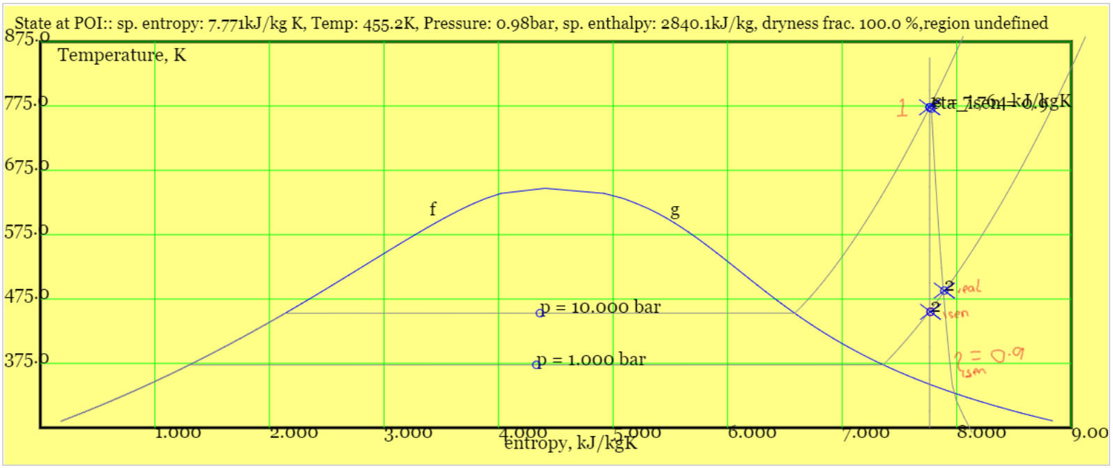
Example 3B.050: Steam is fed to an axial turbine at \(T_1=773K, \; p_1=10 bar\) and a flow rate of \(\dot{m}=5kg/s \). The exit pressure is \(p_2 = 1 bar \). Estimate the derived power for (1) an isentropic process (2) a process with an isentropic efficiency of 90%.
For steam-driven turbine, the isentropic condition, \( s_1 = s_2 \), allows a first guess of the outlet state.
Problem Statement: Isentropic and anisentropic power production by a steam turbine.
Schematic: See sketches for Example 3B.030. A TS diagram will be produced in the discussion section.
Assumptions: Steady conditions - no accumulation (storage) of energy in the turbine. Ignore heat transfer to the turbine (hence \(\dot{Q}=0\)) in SFEE. Ignore changes in gravitational potential energy and kinetic energy. Initially an isentropic process.
Physical Laws: First Law in form of SFEE with gravity terms eliminated. Use of IAPWS properties.
Calculation: First obtain the isentropic exit temperature.
I used my own interactive graph, please see the screen shot below. The 1 bar isobar, 10 bar isobar and start point (point 1) were input via keyboard. The isentropic end point was selected by eye, with minor errors. At the turbine inlet
$$h_1=3479 kJ/kg \quad s_1=7.764 kJ/kgK $$
At the outlet there are minor errors in entropy and pressure,
$$ h_{2,isen} = 2845 kJ/kg \quad s_2 = 7.763 kJ/kgK \quad p_2 = 1.02 bar $$
The isentropic power is,
$$ \dot{W}_{t,isen} = \dot{m}({h_{2,isen}-h_1}) = 5 \times (2845-3479) = -3\;170 kW $$
The real-world power is,
$$ \dot{W}_{t} = \eta_{isen} \dot{W}_{t,isen} = 0.9 \times (-3\;170 ) = -2\;853 kW $$
Or use the "irreversible expansion" button to draw the "real expansion, crossing the
1 bar line at \( h_2=2899 kJ/kg \) and
$$ \dot{W}_t = \dot{m}{h_{2 }-h_1} = 5\times(2899-3479)=-2 \; 900 kW $$
Discussion: My enthalpies are within 2kJ of values in the Rogers and Mayhew Steam Tables.
The Ts diagram is plotted below. The straight vertical line from 1 to 2-isen represents the isentropic expansion. The slanted curve from 1 to 2-real is the real-world expansion.
A reheater is frequently employed between "high pressure" and "low pressure" turbines.
Cycles using reheaters tend to be more efficient and tend to generate more work per unit mass of working fluid. A further advantage in steam cycles is that exhaust steam is drier, or completely dry, thereby reducing the erosion of blades. An example of a reheater configuration is a bundle of fire tubes with combustion gases on the outside and steam on the tube-side. For preliminary calculations on the reheater, one removes from the SFEE (Equation 4) shaft power, kinetic energy and potential energy terms. The heating power is equal to enthalpy change,
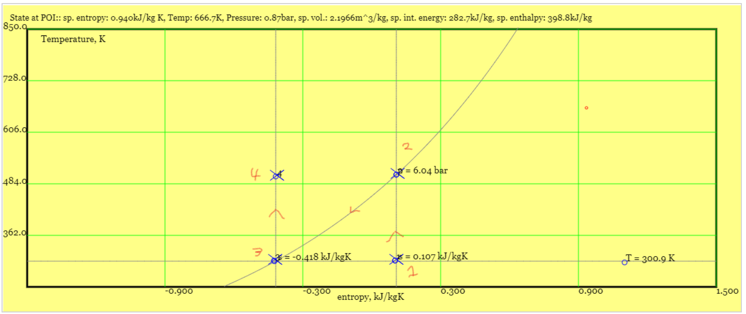
Figure 4: Two turbines with an intermediate reheater (a) Plant diagram showing high pressure turbine (1-to-2), intermediate reheater (2-to-3) and low pressure turbine (3-to-4)(b) pV plot (c) Ts plot
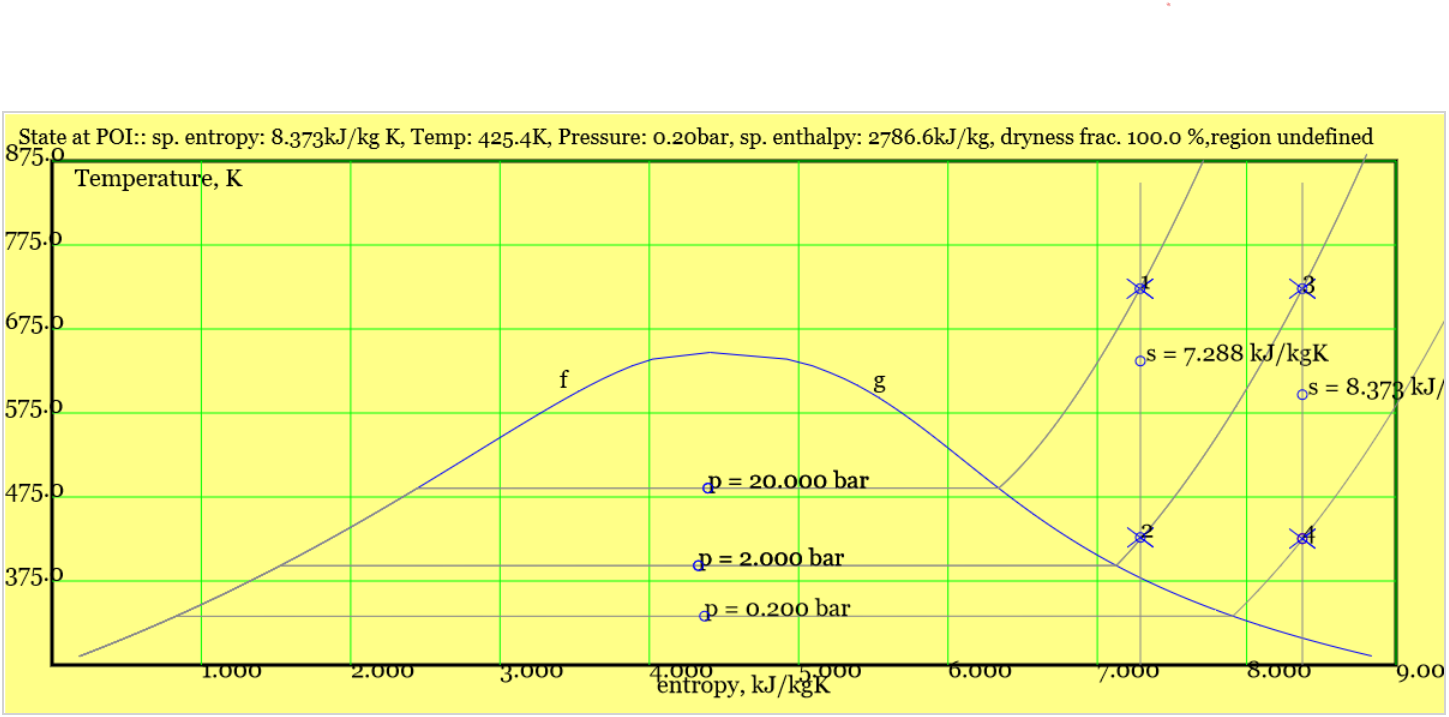
Example 3B.060: Steam is fed to an axial turbine at \(T_1=723K, p_1=20 bar\) and a flow rate of \(\dot{m}=2.4 kg/s \). The steam is expanded isentropically (at constant entropy) in a high pressure turbine to 2 bar, and then reheated to 723K. The steam is then further expanded isentropically in a low pressure turbine to 0.2 bar. Estimate the derived power from each turbine and the required heating power for the reheater.
Reheating gives better specific turbine work and maintains steam dryness.
Problem Statement: Power production from steam turbines with reheat.
Schematic: See sketches in Figure 4.
Assumptions: Steady conditions - no accumulation (storage) of energy in the turbines and reheater. Ignore heat transfer to the turbine (hence \(\dot{Q}=0\)) in SFEE. Ignore changes in gravitational potential energy and kinetic energy. Isentropic process. Ignore pressure losses across the heater and any work against friction in the heater (\( \dot{W}_s = 0 \)).
Physical Laws: First Law in form of SFEE with gravity terms eliminated. Use of IAPWS properties.
Calculation: First obtain the enthalpies and entropies at the four points.
I used my own interactive graph, please see the screen shot below. At 1,
$$T_1=723K, p_1=20 bar \implies h_1= 3357.7 kJ/kg, s_1 = 7.286 kJ/kgK $$
At 3
$$T_3=723K, p_3=2 bar \implies h_3= 3381.2 kJ/kg , s_3 = 8.373 kJ/kgK $$
At 2
$$ s_2=s_1, p_2=2bar \implies h_2 = 2776.3 kJ/kg $$
At 4
$$ s_4 = s_3, p_2 = 0.2bar \implies h_4 = 2786.6 kJ/kg $$
The derived power from the two turbines is,
$$ \dot{W}_{12} = \dot{m} (h_2-h_1) = 2.4 \times (2776-3358) = -1\;397 kW $$
$$ \dot{W}_{34} = \dot{m} (h_4-h_3) = 2.4 \times (2787-3381) = -1\;426 kW $$
The heating power is
$$ \dot{Q}_{23} = \dot{m} (h_3-h_2) = 2.4 \times (3381-2776)= 1\;452 kW $$
Discussion: (1) The three energy transfers are within 4% of each other.(2)The output from the interactive graph is shown below. All steam is dry. Were the isentropic expansion from 20bar to 0.2bar acheived in a single turbine, the exit steam would be wet with quality \(x=0.91\).
For a single turbine, expanding to 0.2bar, the interactive graph tells me \(h_2 \approx 2393kJ/kg\) and from the SFEE
\( \dot{W} \approx -2\;316 kW \) versus \( -2\;823 kW \) from the reheat scheme. Reheat gives more work per unit mass of steam.
In the above example, the three energy transfers are within 4% of each other. The same conditions applied to an ideal gas would yield identical energy flows. The two isentropic turbines are characterised by equal pressure ratios , \( r_p = p_1/p_2 = p_3/p_4 = 10 \) and equal inlet temperatures \(T_1=T_3\). For an ideal gas turbine exit temperatures are also identical, viz.
And the temperature difference used to obtain \(\dot{Q}_{23}\) is the same, that is
\( T_3-T_2 = -1 \times (T_2-T_1) \) and \( \dot{Q}_{23} = -1 \times \dot{W}_{12} \).
Finally, is useful to reflect carefully on the difference between the moving boundary work in a closed system and shaft work in an open system. There are two issues in particular with the pressure volume curve. Firstly, for an open system the x-axis would normally refer to specific volume, and the process thereon describes one unit mass passing from 1 to 2. (Specific means "per unit mass".) The area under the p-v curve represents total specific work \(w\); this is the total of shaft work provided by expansion plus two pieces of flow work.
$$ w = -\int_1^2 p dv = w_s + w_{b1} + w_{b2} = w_s + p_1 v_1 - p_2 v_2 $$
Rearrange to obtain the shaft work,
\begin{equation}
w_s = -\int_1^2 p dv + p_2 v_2 - p_1 v_1 = -\int_1^2 p dv + \int_1^2 d(pv) = \int_1^2 v dp
\end{equation}
For an open system shaft work is the area to the left of curve 1-2. Or, if the plot is appropriately rotated and reflected, shaft work is the area under the v-p curve. This additional information is useful for non-adiabatic systems, \( \dot{Q} \ne 0 \).
5.) Compression of Gas - Diffusers and Compressors
Compression of a gas is associated with increased pressure and increased enthalpy. It is the opposite of expansion.
Diffusers increase pressure by deceleratating fluids. They are found at jet engine intakes or (when termed a "tail race") on the outlet end of water turbines. For the purposes of a year 1 or year 2 undergraduate course, their shape is imagined as a reflection of a simple nozzle. (Real world diffusers can be far more complex than this.)
A compressor raises gas pressure several fold (as opposed to fans and blowers, which raise pressures by a few kPa). The machine, internals need not concern us excessively here (an axial compressor has alternating arrangements of rotors and stators).
Figure 5: Components that compress a fluid. (a) Diffuser (b) Compressor.
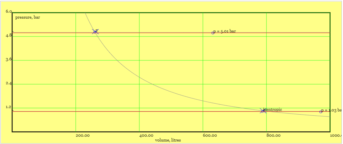
Example 3B.070: A compressor acts and processes \( 2 kg s^{-1} \) of air. Input conditions are \(T_1 = 293 K, \; p_1 = 1 bar\). At the outlet \( p_2 = 5 bar\). Find the power requirement for isentropic compression, and compression with an
isentropic efficiency of 70%.
The isentropic condition allows a first guess of the outlet state of a compressor.
Problem Statement: Power input for isentropic compression.
Schematic: See sketches in Figure 5(b).
Assumptions: Steady conditions - no accumulation (storage) of energy in the compressor. Ignore heat transfer to the compressor (hence \(\dot{Q}=0\)) in SFEE. Ignore changes in gravitational potential energy and kinetic energy. Isentropic process (for first part).
Physical Laws: First Law in form of SFEE with gravity terms eliminated. Ideal gas properties and laws.
Calculation:
Use isentropic relationships to get the outlet temperature,
$$ T_2 = T_1 (\frac{p_2}{p_1})^{(\gamma-1)/\gamma} = 293 \times (5/1)^{2/7} = 464K$$
$$ \dot{W}_{c,isen} = \dot{m}(h_2-h_1) = \dot{m}c_p(T_2-T_1) = 2 \times 1.005 \times (464-293)kW $$
$$ \dot{W}_{c,isen} = 344 kW $$
Note that this is an ideal energy requirement, and it makes sense that the real world power requirement will be
greater . It is necessary to divide by isentropic efficiency (see discussion below in the main text).
$$ \dot{W}_c = \frac{\dot{W}_{c,isen}}{\eta_{c,isen}} = \frac{344}{0.7} = 491 kW $$
Discussion: The process is sketched below on a pv diagram (the x-axis represents specific volume). From inspection by eye \(h_1 \approx 19kJ/kg \quad h_2 \approx 187 kJ/kg \) and the isentropic work is \( \dot{W}_{c,isen} = 2 \times (187-19) \approx 336 kW \). Note that because an open system
is considered the specific power is the area to the left of the curve.
The isentropic efficiency of a compressor puts real work on the denominator; for turbine efficiency the real work appears on the numerator.
The above example concerns an isentropic compression: there is no heat transfer to the fluid and no gas friction. For smaller compressors, typically used in the teaching laboratory, automotive workshop or domestic refrigerator, heat transfer can be substantial - indeed the casings of reciprocating compressors usually incorporate fins to encourage cooling of the unit. In large power production plants or engines the heat transfer might be small but nonetheless gas friction is important. Again, an isentropic efficiency relates the "ideal" isentropic power to the real world power. Let \(w_f\) be the specific friction work, required to overcome gas friction.
$$ w_c = w_{c,isen} + w_f $$
For the compressor the isentropic efficiency is the
ratio of isentropic work to real work.
With reference to the corresponding equation for a turbine, the numerator and denominator have been exchanged. Arithmetically, this is because efficiency should be a number between zero and one, friction work is always positive, turbine work is negative and compressor work is positive.
The power demanded by compression is reduced by intercooling . The compression is staged, and, In the simplest system, a cooler is placed between two compressors. Theoretically, the minimum power of compression would be demanded by isothermal exansion (or, an infinite series of compressors with intercoolers).
Figure 6: Two compressors with an intermediate cooler (a) Plant diagram showing low pressure compressor (1-to-2), inter-cooler (2-to-3) and high pressure compressor (3-to-4)(b) pV plot (c) Ts plot
Example 3B.080: Air at 300K is to be compressed isentropically from 1 bar to
36 bar. Estimate the necessary specific work for (1) a single compressor (2)
two intercooled compressors with equal pressure ratio. The intercooler reduces the pressure of medium pressure air to 300K.
Intercoolers reduce the power needed for compression.
Problem Statement: Power input for staged compression with intercooling.
Schematic: See Figure 6 above.
Assumptions: Steady conditions - no accumulation (storage) of energy in the compressor(s). Ignore heat transfer to the compressor(s) (hence \(\dot{Q}_c=0\)) in SFEE. Ignore changes in gravitational potential energy and kinetic energy. Isentropic processes.
Physical Laws: First Law in form of SFEE with gravity terms eliminated. Ideal gas properties and laws.
Calculation: For a single compressor with a pressure ratio a 36:1 then the exit temperature follows from,
$$ T_2 = T_1 (p_2/p_1)^{(\gamma-1)/\gamma} = T_1 r_p^{2/7} =835K$$
Applying the SFEE
$$ w_{12} = c_p (T_2-T_1) = c_p T_1 (r_p^{2/7}-1) $$
$$ w_{12}=1.005 \times 300 \times 300 \times (36^{2/7}-1) = 537 kJ/kg $$
For the intercooled system the two compressors both have a pressure ratio of \( \sqrt{36/1}=6\). Then
$$ T_2 = 300 \times 6^{2/7} = 501 K \qquad isentropic \; process \; with \; r_p=6$$
$$ T_3=T_1 = 300K \qquad specified $$
$$ T_4=T_2 \qquad same \; pressure \; ratio $$
For the above conditions,
$$ w_{tot} = w_{12}+w_{34} = c_p(T_2-T_1+T_4-T_3)=2c_p(T_2-T_1)=404kJ/kg$$
The specific heat transfer in the intercooler is,
$$q_{23} = c_p(T_3-T_2) = -1 \times c_p(T_2-T_1) = -w_{12} = -202 kJ/kJ.$$
And the temperature of gas leaving the system is \( T_4=501K \).
Discussion: The very large pressure ratio makes the pV curve difficult to read. The Ts diagram is easier and a screendump from my
interactive chart is shown below. By eye, \(h_1=33kJ/kg; \; h_2=239kJ/kg; \; w_{12} = 239-33=206kJ/kg \), close to above calculations.
An analysis of isothermal compression provides a useful limit - this would require an infinite sequence of compressors/ intercoolers. For isothermal flow work (see Equation 7),
$$ w_s=\int^2_1 v dp = RT \int^2_1 \frac{dp}{p} = RT \, ln (p_2/p_1) = 0.287 \times 300 \times ln(36) = 309 kJ/kg $$
6.) Throttling - the Isenthalpic Process
A frictional obstruction, such as a partially closed valve, serves to reduce the pressure of a flow with minimal enthalpy change. Isenthalpic means "same enthalpy".
Throttling is often associated with a change in phase. Throttles are employed in refrigerators and "flash evaporators" to reduce pressure substantially. The
throttling calorimeter
is employed to measure the dryness of steam. The throttle might be a partically closed valve, a long section of capillary tube, or a porous plug. There is little opportunity for shaft work, and heat transfer and potential energy can reasonably be neglected. The change in kinetic energy is, in practice, far smaller than the enthalpies of phase change experienced in refrigerators and power plant. The only terms to remain in the SFEE are enthalpy.
$$ 0 = \dot{m}(h_2-h_1) \implies h_2 = h_1 $$
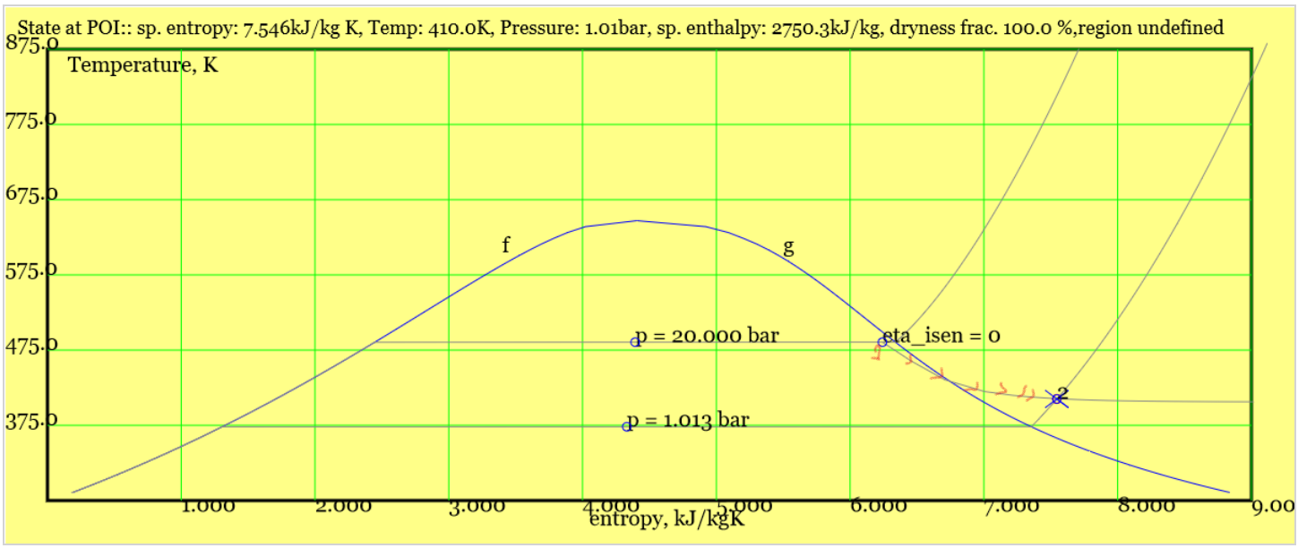
Example 3B.090: Steam at 20bar passes through a throttle, exiting at \(p_1=1.013bar, T=410K\). Estimate the dryness fraction of the original steam.
Problem Statement: Dryness fraction of steam at 20bar, indicated by a throttling calorimeter.
Schematic: I used my interactive graph to get check my solution (see discussion below).
Physical laws: First Law, leading to Steady Flow Energy Equations. IAPWS steam properties.
Calculation:
At 2 $$ p_2 = 1.013 bar, T_2 = 410K \implies h_2 = 2750.3 kJ/kg $$
At 1 $$ p_1=20 bar, h_f=909kJ/kg, h_g= 2798kJ/kg, h_1=h_2= 2750 kJ/kg $$
From the
wet vapour relationships,
$$ h_1=h_2 = x \, h_f +(1-x) \, h_g$$
$$ 2750 =909 x + 2798 (1-x) \implies x=97.5\;per\;cent$$
Discussion: This sort of dryness fraction is typically experienced at the exit of some turbines. On the interactive graph,
I checked my calculation using an isenthalpic efficiency of zero (I sharted at point 1 with x=0.975, and the expansion crosses the low pressure isobar at the expected \(T_2=410K\).
7.) Mixing Chambers
For example, let us apply the multistage version of the SFEE (Eqn 5) to a domestic show with integral water mixing unit.
Very hot water and cold water are mixed to produce water at a comfortable temperatures. There are
three streams (two in, one out). Terms include shaft power for the pumps, any heat transfer from electrical elements,
and water enthalpy. Kinetic and potential energy terms are neglected.
8.) Heat Exchangers
The purpose of a heat exchanger is to transfer heat from one fluid stream to
another fluid stream without allowing the two to mix.
The simplest conceivable heat exchanger is arguably the fire tube within a steam engine. Hot gases on
the inside of the tube pass their energy to the external water and steam. The automotive radiator is another example of a conceptually simple system - hot water on the inside of a tube transfers heat to an external air flow. (Conceptually similar air-cooled heat exchangers exist at large industrial scale.)
The combustion chamber in a jet engine is not a heat exchanger. Nor is the fuel injector system for a reciprocating engine. Nonethless, simplified thermodynamic treatments refer to "heat addition" - that is, the combustion chamber is treated in the same way as a heat exchanger. (This works as a first approximation because the specific heat capacity of exhaust gase is close to that of air.)
In open systems, heat exchangers are employed to recover exhaust heat from turbine exhaust and offset some of the energy input that would otherwise be required in the combustor. There are two streams - exhaust gas and clean air. The simplest
concept is the
"concentric pipe" or "pipe-in-pipe exchanger .
Heat transfer and heat exchangers will be considered in detail in a later note . For the time being, it suffices
to define the concept of effectiveness . Each stream has a heat capacity flow, \( \dot{m} c_p \). The effectiveness refers to the stream with the lowest heat capacity flow. (When the two streams have equal heat capacity flow the effectiveness can apply to either stream.)
$$ e = \frac{change \; in \; specific \; enthalpy \; of \; stream \; with \; lowest \; capacity \; flow}
{maximum \; possible \; specific \; enthalpy \;change \; in \; that \; stream} $$
For an ideal gas or pure fluid,
$$ e = \frac{T_{in}-T_{out}}{T_{in}-T_{max/min} } \qquad \; stream \; with \; lowest \; heat \; capacity \; flow $$
Term \(T_{max/min} \) is the maximum or minimum possible temperature at outlet. It is equal to the temperature of the adjacent stream.
Example 3B.100: Hot exhaust gas emerges from an incinerator at \(120 ^oC \). This passes through a serpentine loop, cooled by spraying very large amounts of cold water at onto the loop's external surface. The loop is configures such that were it infinitely long the exit gas temperature would be equal to that of the water, \(20^oC\). The loop is certainly not
infinitely long, and has an effectiveness of 65%. Estimate the exit temperature of the exhaust gas and (assuming that the gas has similar properties to air) estimate the specific heat transfer.
Effectiveness tells us exit temperature and heat transfer rate.
Problem Statement: Cooling power supplied to an exhaust gas plus gas exit temperature.
Schematic:
Assumptions: Steady conditions - no accumulation (storage) of energy in the cooling loop. Ignore and fan power (hence \(\dot{W}_s=0\)) in SFEE. Ignore changes in gravitational potential energy and kinetic energy. Assume the exhaust gas has
the same heat capacity as air, \(c_p = 1.005 kJ/kg K \).
Physical Laws: First Law in form of SFEE. Use of effectiveness definition.
Calculation:
Using the above expression for effectiveness
$$ e = \frac{T_{in}-T_{out}}{T_{in}-T_{max/min} } $$
The minimum theoretical outlet temperature would be equal to the water temperature, \( T_{min}=20^oC\).
$$ 0.65 = \frac{120-T_{out}}{120-20} \implies T_{out} =55^oC$$

 For a single turbine, expanding to 0.2bar, the interactive graph tells me \(h_2 \approx 2393kJ/kg\) and from the SFEE
\( \dot{W} \approx -2\;316 kW \) versus \( -2\;823 kW \) from the reheat scheme. Reheat gives more work per unit mass of steam.
For a single turbine, expanding to 0.2bar, the interactive graph tells me \(h_2 \approx 2393kJ/kg\) and from the SFEE
\( \dot{W} \approx -2\;316 kW \) versus \( -2\;823 kW \) from the reheat scheme. Reheat gives more work per unit mass of steam.
 An analysis of isothermal compression provides a useful limit - this would require an infinite sequence of compressors/ intercoolers. For isothermal flow work (see Equation 7),
$$ w_s=\int^2_1 v dp = RT \int^2_1 \frac{dp}{p} = RT \, ln (p_2/p_1) = 0.287 \times 300 \times ln(36) = 309 kJ/kg $$
An analysis of isothermal compression provides a useful limit - this would require an infinite sequence of compressors/ intercoolers. For isothermal flow work (see Equation 7),
$$ w_s=\int^2_1 v dp = RT \int^2_1 \frac{dp}{p} = RT \, ln (p_2/p_1) = 0.287 \times 300 \times ln(36) = 309 kJ/kg $$