These notes concern the dynamics of gases in nozzles - that is in ducts with changing cross-sectional area. A simple converging nozzle will accelerate a gas by constricting flow, and thereby produce thrust: rockets that exploit this principle have been around for centuries. There are, however, some intricate aspects of gas dynamics. If we are dealing with liquids, it is not unusual to assume a constant temperature (and internal energy), and Bernoulli easily relates flow work to kinetic energy. In gases acceleration leads additionally to expansion and cooling. For Mach numbers exceeding a limit in the range 0.1 to 0.3 there is an appreciable change in Thermodynamic properties - pressure, temperature and density. Moreover, in a simple converging nozzle the maximum velocity in the exit plane is limited to the local speed of sound in still gas; there is a corresponding maximum possible rate of mass flow. This mass flow cannot be increased by adding to the nozzle. Nonetheless, an additional diverging section encourages rapid increases in the specific volume of the gas leading to gas velocities that exceed the sonic value. I find this observation surprising and counterintuitive: gases at supersonic speed are accelerated by increased cross-sectional area.
Simple analytical solutions assume that flow is isentropic - in effect, adiabatic and frictionless. In supersonic flows, some frictional effects occur in very thin zones known as shocks. The "sonic boom" is well known to the general public. The effect of a shock is always to decelerate and compress the flow.
I intend the content to be suitable for Year 1 and Year 2 students of General/ Mechanical and Chemical Engineering. Students of Aerospace Engineering may well require further information.
2. Introduction
These notes concern principally the mass flow and thrust produced by nozzles. I intend to get the reader far enough
to understand how tabulated quantities of isentropic flow and normal shocks are derived, and applied to simple topics. Note that a nozzle is limited by the speed of sound at its narrowest point - the gas here cannot exceed this velocity. Note also that analytical solutions are often expressed as functions of the dimensionless Mach number- the quotient of velocity and the local speed of sound in still gas. The notes are intended to assist the reader to be able to:
explain the speed of sound and appreciate how it may be derived;
describe the observe performance of converging and converging-diverging nozzles;
describe "choking";
appreciate how the conservation of mass, momentum and energy applies to isentropic flows and shocks;
use equations, tables or both to solve simple problems relating to nozzle areas and changes in flow properties.
The text includes my own versions of the isentropic Flow Tables and Normal Shock tables. The increments of Mach number are comparatively large, in the interests of readability. In the fullness of time I intend to publish more granular tables as separate web pages.
The reader is assumed to have studied the following topics:
These notes do not deal with the shape of a nozzle. (A badly shaped nozzle will create
unnecessary internal expansion and compression waves.) This topic used to be tackled by graphical
analysis - see for example
Crown's NACA report in the US archives.
3. The speed of sound
A pressure signal moves with finite velocity and will accelerate a gas.
The speed of sound in an ideal gas is written as
$$ a = \sqrt{-v^2 (dp/ dv)_s} = \sqrt{\gamma R T} \qquad (1) $$
where a is the speed of sound, p is pressure, v is specific volume, R is the specific gas constant, T is temperature, \( \gamma \) is the ratio of heat capacities, and the subscript s indicates an isentropic process.
When the gas velocity exceeds 10 to 30% of sonic velocity a, the gas flow will be associated with appreciable changes on pressure, density and temperature. Very high gas velocities are required on jet engines so as to produce thrust.
Here is my own thought experiment that demonstrates the effects of compressibility on density and momentum. It can be used to prove the above Equation 1. Consider a piston-cylinder initially with both its gaseous contents and the piston stationary, and the piston front face on surface A-A. A microphone located on surface B-B lies upstream of the piston face. At time t=0 the piston accelerates instantaneously to a very low velocity du. Consequently velocity du and a pressure p + dp is confined to an infinitesimally thin gas layer touching the piston face - see the red section of line A-A on part (a) of Figure 2. Gas to your right hand side of AA is stationary and at pressure p. A finite time, \( \tau\), elapses
before the microphone detects any pressure rise at BB and the gas at BB moves at velocity du. At this time the piston has moved from AA to CC, and in zone CC-BB all gas exhibits p+dp and du (see red rectangle in part (b) of Figure 2). Gas to your right hand side of BB is still stationary and and at pressure p. Figure 2(c) shows a plot of pressure at BB - note the step change at time \( t = \tau \). From a reference point upstream of the microphone the pressure wave has travelled at the speed of sound,
$$ a = \frac{length \; AB}{\tau} $$
Figure 1 Schematic representation of the speed of sound (a)at time t=0 piston at AA instantaneously accelerated to velocity du and face pressure p+dp, affecting an infinitessimally thin section of gas (red line) (b)
at t=tau, piston has advanced to CC whereas affected gas (red) occupies CC to BB at velocity du and pressure p+dp (c) pressure versus time at BB .
I emphasise that at time \(t = \tau \) no gas has passed through BB and the gas upstream of BB holds its original pressure p and zero velocity. (At \( t \gt \tau \) the sound wave continues to travel further along the cylinder at the sonic velocity a.)
Imagine now the piston-cylinder to be mounted laterally on a trailer, moving with velocity u. The velocity of the sound wave is still velocity a relative to downstream gas in the cylinder, but to an observer on the roadside it is \(a \pm u\). Here is another example: suppose I hear a rifle shot on a windy day when the speed of sound in still air would be 330m/s and the wind speed is 20 m/s. Depending on my position the sound will reach me at a velocity between 310 and 350/s.
3.1 Derivation of the Speed of Sound
Sound compresses slightly a gas, thereby reducing its specific volume
Let us treat movement of the piston face from AA to CC as part of a moving boundary problem
( Figure 2, parts (a) and (b)). So long as line BB bounds a closed system
( true if \( t \leq \tau \) ) gas to the left of BB is compressed. The volumes swept by the piston face (dV) and the sound wave (V) are both in
proportion to their velocities .
The gas experiences a
volumetric strain,
$$ dV/V = -du/a $$
Because the mass m inside the closed system is constant the specific volumes are \( dv = dV/m \) and \( v = V/m \). Then with algebraic manipulation,
$$ du = - a dv/ v \qquad (2) $$
Sound acts to accelerate slightly the gas
The mass from piston face to BB, coloured red in Figure 2b, has been accelerated from rest to velocity du. Newtons Second Law equates a force to the product of mass and acceleration. The gas mass in the closed system is constant, and most easily calculated at the initial time t=0,
$$ m = \frac{length \; AB \times A}{v} = \frac { a \tau A}{v} $$
where A is the area of the piston face. The net force action on the gas is \(F_{net} = A dp \), and the acceleration is \( acc = du/\tau \). Substitution for force, mass and acceleration yields the
Joukowski equation ,
$$ F_{net} = m \times acc \implies dp = a \frac {du}{v} \qquad (3) $$
(It is useful for analysis of water-hammer and Bosch's 'measurement of fuel injection' by means of a rate tube.)
Combine Equations 2 and 3 to eliminate du and yield the sonic velocity, a. So long as dp is very small we can specify an isentropic processes
$$a = \sqrt {-v^2 (\frac{dp}{dv})_s }\qquad (1) $$
The solution can be developed in several ways
In terms of the bulk modulus, \( \kappa \) (the applied pressure difference per unit volumetric strain),
$$ a = \sqrt {\kappa \, v} \qquad where \; \kappa = -v dp/dv \qquad 4a $$
For an isentropic ideal gas process where \( p v ^ {\gamma} = const \implies dp/dv = -\gamma p/v \)
$$ a = \sqrt {\gamma pv } \qquad ideal \; gas \; \qquad 4b $$
The above can be written in terms of temperature, noting the Ideal Gas Law \( pv = RT \),
$$ a = \sqrt {\gamma RT } \qquad ideal \; gas \; \qquad 4c $$
The well-known Mach Number is the ratio of velocity to sonic velocity. Thus,
$$ M = \frac{c}{a} \qquad 4d $$
Then for an ideal gas it is useful to note, from Equations 4c and 4d,
$$ c = M \sqrt {\gamma RT} \qquad ideal \; gas \; \qquad 4e $$
4. Flows in Nozzles
Nozzles produce thrust or accelerate gases in turbo-machines. The cross sectional area of the nozzle changes with distance downstream. I shall start with the theory for simple, converging nozzles. This is largely applicable to more complicated Converging-Diverging (or De Laval) nozzles. As well as producing thrust and propulsion directly, nozzles feature inside turbo-machinery and in process engineering.
4.1 Converging nozzles
A converging nozzle generates thrust by accelerating a gas and increasing its momentum.
Converging nozzles were used in rockets
until the 19th century .
Their investigation is a useful pre-requisite to a study of converging-diverging nozzles.
Consider a nozzle fed from a reservoir. There are four pressures of particular interest. The reservoir exhibits the greatest pressure, \(p_o \). So long as the reservoir is big enough to ensure that flow velocity is close to zero, the pressure therein is known variously as reservoir, stagnation or total pressure. The next pressure of interest is in the exit plane of the nozzle, \( p_{exit}\). Throughout the surroundings, which extend to typically a millimetre of the exit plane, the back pressure holds, \(p_{back}\). If the back pressure exceeds a critical value, \(p_{back} \gt p_{crit} \), then it is equal to the pressure in the exit plane. The thrust developed by the nozzle is then equal to the rate of change of gas momentum. Given that a rocket nozzle accelerates propellants from zero velocity to the velocity in the exit plane, the thrust is
$$ Thrust = \dot{m} c_{exit} \qquad p_{back} \ge p_{crit} \qquad 5a $$
Note that velocity c is relative to the rocket engine. At lower back pressures,
$$ Thrust = \dot{m} c_{exit} + A_{exit} (p_{exit}-p_{back}) \qquad p_{back} \le p_{crit} \qquad 5b $$
This leaves us with the tasks of computing the velocity, specific volume, and mass flow in the exit plane (see next section).
Let us take the full set of properties of interest in the reservoir as \(p_o, T_o, h_o, v_o, \;\) and velocity \( c_o=0 \). It has been observed that the exit velocity cannot exceed the local velocity of sound in still air. (Any further reduction in back pressure will not "communicate" to the reservoir, because the net gas velocity relative to the exit plane is zero.) Let us conduct a thought experiment in which the back pressure is reduced gradually from \(p_{back}=p_o\) to \(p_{back}=0\).
\(p_{back} = p_o \) : the pressure is constant throughout the duct and gas is stationary;
\( p_o \gt p_{back} \gt p_{crit} \): the pressure and temperature decrease along the duct. The the back pressure holds from the nozzle exit plane to the far field - some distance downstream of the exit plane. Gas accelerates along the duct reaching its maximum velocity at the duct exit. At no point does the gas achieve sonic velocity.
\(p_{back}=p_{crit}\): the back pressure is equal to the critical pressure. At this stage gas achieves the speed of sound in the exit plane.The mass flow rate of gas can be increased no further and the nozzle is said to be choked . All other observations are as above.
\(p_{back} \lt p_{crit}\): The nozzle is choked. The speed of sound is achieved in the exit plane. Further reductions of back pressure below its critical value have no effect of the pressures, velocities and temperatures inside the nozzle. A rapid expansion and depressurisation of gas, evident a short distance beyond the exit place, is not isentropic and has a three-dimensional flow.
Figure 2 Pressure profiles along a converging nozzle
4.2 Isentropic acceleration of a gas
In acceleration, the conversion of enthalpy to kinetic energy reduces temperature. There is an isentropic relationship between temperature and pressure at any point .
To calculate thrust, we need to know fluid properties along the nozzle and especially at the exit plane. I'll introduce the problem here using "primitive" variables. In the next section I'll introduce the dimensionless forms commonly listed. The principles at play are: mass conservation, energy conservation (the SFEE), and the isentropic relationships. The following assumptions are commonly made,
flow is steady;
flow is one dimensional - there is no radial variation in velocity or pressure;
there is no transfer of work or heat between the surroundings and the flow;
processes are thermodynamically reversible - in the absence of heat transfer a reversible process is also an isentropic process and isentropic relationships are applicable;
ideal gas behaviour is often assumed (enabling use of \( pv = RT \) ).
the gas velocity in any reservoir feeding the nozzle is small enough to be ignored.
Let us start by taking the pressure, p, at a given location in the nozzle as known. Then the temperature follows from the isentropic relations,
$$ s = const. \implies T= T_o (\frac{p}{p_o})^{(\gamma-1)/\gamma} \qquad 6 $$
For a steady, one-dimensional flow with no heat and work transfer the Steady Flow Energy Equation becomes,
$$ h_o = h + \frac{c^2}{2} \qquad 6b $$
For an ideal gas, \( h= c_p T \) and thus velocity and temperature are related by,
$$ c = \sqrt { 2 (T_o-T) c_p} \qquad ideal \; gas \qquad 7 $$
the mass flow rate at any plane of interest is,
$$ \dot{m} = \frac {A c}{v} \qquad 8 $$
where A is cross sectional area, and v is specific volume.
Example CF0010 A reservoir holds air at pressure \(p_o= 10 bar \) and temperature \(T_o = 300K \). Estimate the rate of mass flow through the nozzle and the thrust generated when the pressure in the exit plane is \(p_{exit} = 7.08 bar\). The area of the nozzle exit is \(1.0 \times 10^{-4} m^2\).
Solution:
Problem statement: Find the mass flow rate and thrust in a converging nozzle for specified pressures
Diagrams: See Figure 2, and in particular curve 2.
Assumptions: The flow is not choked. Assumptions 1-6 in Section 4.2 above.
Physical laws: Mass conservation; energy conservation in form of SFEE, relating velocity and temperature changes; isentropic expansion, relating temperature and pressure.
Calculation:
From the isentropic T,p relationship, Equation 6, the temperature in the exit plane is,
$$ T_{exit} = 300 \times (\frac{7.08}{10})^{2/7} = 271.8 K $$
From the adapted version of the SFEE, Equation 7,
$$ c_{exit} = \sqrt { 2 (300-271.8) \times 1005} = 238.1 m/s$$
Before we find the mass flow rate we need the specific volume of air at the local temperature and pressure in the exit plane. The Ideal Gas Law gives,
$$ v = \frac{R T_{exit}}{p_{exit}} = \frac{0.287 \times 271.8}{708} =0.1102 m^3/kg$$
From Equation 8 the mass flow rate is,
$$ \dot{m} = \frac {A_{exit} c_{exit}}{v_{exit}}= \frac { 1.0 \times 10^{-4} \times 238.1}{0.1102} = 0.2161 kg/s$$
There is no change in pressure so the thrust is,
$$ Thrust = \dot{m} c_{exit} = 238.1 \times 0.2161 = 51.4 N $$
To check, let us find the speed of sound in the exit plane,
$$ a_{exit} = \sqrt{\gamma R T_{exit}} = \sqrt {1.4 \times 287.1 \times 271.8} = 330.5 m/s $$
We then get values for the following dimensionless groups
$$ M_{exit} = \frac{c_{exit}}{a_{exit}} = \frac{238.1}{330.5 } =0.7204 $$
$$ \frac{T}{T_o} = \frac{271.8}{300} = 0.906 $$
$$ \frac{p}{p_o} = \frac{7.08}{10} = 0.708 $$
To within three significant figures, the calculated values of Mach number, temperature ratio and pressure ratio in example CF0010 agree with the calculator in Table 1 (at the end of the next section), and with estimates in published
Isentropic Flow Tables . We shall discuss shortly the ratio \(A/A*\).
It is sometimes useful to relate temperature to Mach number rather than velocity. Recall the definition of Mach number (Equation 4e) and the modified version of the SFEE (Equation 7)
$$ c = M^2\sqrt{\gamma R T } \qquad (4e) \qquad \qquad c = \sqrt { 2 (T_o-T) c_p} \qquad \qquad (7) $$
Then eliminate velocity c to get,
$$ T = \frac{2 T_o}{2 + M^2\gamma R/ c_p} \qquad (8b)$$
This will be developed further in the next section.
For a hypothetical second nozzle working with an identical rate of mass flow, an area A* is the theoretical exit plane area that would allow choking. Choking brings the gas to its sonic velocity (at the exit plane in a converging nozzle). Thereupon the velocity is that of sound in still gas. Substitution of M=1 into Equation 8b above gives the corresponding temperature ratio.
Example CF0020 Refer to the previous example (\(p_o= 10 bar \) , \(T_o = 300K \) , \( A_{exit} = 1.0 \times 10^{-4} m^2\) ). A second nozzle is designed (1) to produce the same mass flow rate,
\( \dot{m} = 0.2161 kg/s \),
(2) to accelerate gas to the speed of sound. Find the area of the nozzle exit.
Solution:
Problem statement: Find the exit plane area of a choked converging nozzle.
Diagrams: See Figure 2, and in particular curve 3.
Assumptions: Assumptions 1-6 in Section 4.2 above.
Physical laws: Mass conservation; energy conservation in form of SFEE, relating velocity and temperature changes; isentropic expansion, relating temperature and pressure.
Calculation:
The gas velocity reaches the speed of sound in the exit plane (Equation 4c). It is also predicted by the SFEE (Equation 7).
$$ c_{exit} = a = \sqrt { \gamma R T_{exit}} \qquad sonic \; velocity$$
$$ c_{exit} = \sqrt { 2 (T_o-T_{exit}) c_p} \qquad modified \; SFEE $$
Rearrange the above to eliminate gas velocity,
$$ T_{exit} = T_o \frac{1}{1+ (\gamma R) /2 c_p) } = \frac{300}{1+ 1.4 \times 0.287) /2 \times 1.005} = 250 K $$
(Alternatively, in the next section we find the temperature ratio from either Equation 9 or tables.) Then from the isentropic relationship (Equation 6),
$$ p_{exit} = p_o (\frac{T_{exit}}{T_o})^{\gamma/(\gamma-1)} = 10 \times (250/300) ^{7/2} = 5.283 bar $$
and from the expression for the speed of sound (Equation 4c),
$$ c_{exit} = a_{exit} = \sqrt {\gamma R T_{exit} } = \sqrt {1.4 * 287.1 \times 250 } = 317.0 m/s $$
The Ideal Gas Law yields the specific volume in the exit plane,
$$ v_{exit} =\frac{R T_{exit}} {p_{exit}} = \frac{0.287 \times 250 }{528.3} = 0.1358 m^3/kg$$
Adapting Equation 8 for mass flow rate we get,
$$ A^* = \frac{\dot{m} v}{a_{exit}} = \frac{ 0.2161 \times 0.1358}{317.0} = 0.9258\times 10^{-4} m^2 $$
Note that if we compare the area in example CF0010 with A* then A/A* = 1.080, conforming to the value in Table 1 below and in isentropic flow tables (at M=0.72).
4.3 Published ratios of temperature, pressure and area in isentropic flow
Ratios of temperature, pressure and area versus Mach number are tabulated and published for dry air with \( \gamma=1 \), and can be computed as follows. (Note that most text books show ratios as functions of Mach number only. The equations below demand less algebra and suffice to generate Table 1. )
Equation 8b above usefully relates temperature ratio to Mach number. It is customary to note
the identity
$$ \frac{R}{c_p} = \frac{ \gamma-1}{\gamma} \qquad (8c) $$
and rearrage Equation 8b to obtain the following form.,
$$ \frac{T}{T_o} = \frac{1}{1+ M^2( \gamma-1) /2 } \qquad isentropic \; flow \; of \; ideal \; gas \; (9) $$
Given that the expansion is isentropic so that \( p \propto T^{\gamma/(\gamma-1)} \)
$$ \frac{p }{p_o} = (\frac{1}{1+ M^2(\gamma-1) /2 })^{\gamma/(\gamma-1)} \qquad pressure \; ratio \; (10) $$
The area of the nozzle, A, is related to a hypothetical area A* where, for the same mass flow rate, sonic velocity is achieved and M=1.
$$ \frac{A}{A*}= \frac{1}{M} (\frac { 1+ M^2(\gamma-1) /2 } {1/2+ \gamma /2 }) ^{(\gamma/(\gamma-1))-1/2} \qquad (11) $$
To relate area ratio A/A* to M, start with Equation 8 for mass flow rate and substitute Equation 4e relating Mach number and velocity.
$$ \dot{m} = \frac {A c}{v} = A \frac{M \sqrt{\gamma R T}}{v} $$
Note the isentropic relationship,
$$ v^{-1} \propto T^{1/(\gamma-1)} $$
Then
$$ \dot{m} \propto M A T^{1/(\gamma-1) + 1/2} $$
and to comply with some text books we note that the exponent is equal to,
$$ 1/(\gamma-1) + 1/2 = 1/(\gamma-1) + (\gamma-1)/(\gamma-1) - 1/2 = \gamma/(\gamma-1))-1/2 $$
Now consider a nozzle that is choked. At any position upstream of the exit plane we have arbitrary Mach number, \( 0 \lt M \lt 1\), whereas at the exit plane \(M=1\). Under steady conditions, the same mass flow rate pertains to both locations. Comparing two estimates of the same mass flow rate,
$$ \frac{A}{A*} = \frac{1}{M} (\frac{T(M=1)/T_o}{T(M=any)/T_o}) ^{(\gamma/(\gamma-1))-1/2} $$
To obtain temperature ratios, substitute estimates from Equation 9 with M=any and M=1. Equation 11 then follows.
For the properties of dry air, especially \( \gamma=1.4 \), it is customary and useful to publish tables of the Mach number versus the ratios of area, temperature and pressure. It is also conventional to usefully include the ratio of densities - according to the Ideal Gas law it is the quotient of pressure ratio and temperature ratio. (Note that density is the reciprocal of specific volume.) The tables and the applet in Table 1 include Mach numbers greater than one - see the next section.
Table 1 Tables and calculator for isentropic flow: ratios of temperature, pressure and area versus Mach number.
Heat capacity ratio:
Gamma =
Mach number of interest
M =
To operate, type the heat capacity ratio and the Mach number of interest into the boxes above and click "recalculate". Results for the Mach number of interest are displayed in row 2 with a yellow background.
Example CF0030 A gas bottle of inner volume 73 litres holds 3.650 kg of gas. For the temperature inside the bottle, the speed of sound in still gas is 300 m/s. The bottle experiences a leak, equivalent to a converging nozzle with a circular exit plane of radius 1mm. Estimate the rate of mass loss, in kg/s, if the heat capacity ratio is (1) 1.4 (2) 1.3. Find an approximate check of your solution.
Solution:
Problem statement: Find rate of mass flow through a choked converging nozzle.
Diagrams: See Figure 2, and in particular curve 3.
Assumptions: Assumptions 1-6 in Section 4.2 above. The leak acts in the same way as a converging nozzle. (This forces a high estimate, and for safety-related studies errs on the side of caution.)
Physical laws: Mass conservation; energy conservation in form of SFEE, relating velocity and temperature changes; isentropic expansion, relating temperature and pressure.
Calculation:
Treat the bottle as a reservoir. The density is 3.65/0.073 = 50 kg/m3. Assume that flow is choked in the exit plane so that M=1.
1. γ = 1.4
Look up property ratios at the point of choking,
$$ M=1 \; and \; \gamma=1.4 \implies \; \rho/\rho_o = 0.6339 \implies \rho = 0.6339 \times 50 = 31.7 kg m^{-3} $$
Note that the speed of sound is proportional to \( \sqrt{T} \). In the exit plane,
$$ T/T_o = 0.8333 \qquad \qquad c_{exit}=a_{exit} = 300 \times \sqrt{0.8333} = 274 m/s $$
The area is \( 3.14 \times 10^{-6} m^2 \) and the mass flow rate is,
$$ \dot{m} = c_{exit} \rho_{exit} A_{exit} = 274 \times 31.7 \times 3.14 \times 10^{-6} = 0.0273 kg/s $$
2. γ = 1.3
$$ M=1 \; and \; \gamma=1.3 \implies \; \rho/\rho_o = 0.6276 \implies \rho = 0.6276 \times 50 = 31.4 kg m^{-3} $$
Again, the speed of sound is proportional to \( \sqrt{T} \). In the exit plane,
$$ T/T_o = 0.8696 \qquad \qquad c_{exit}=a_{exit} = 300 \times \sqrt{ 0.8696} = 280 m/s $$
$$ \dot{m} = c_{exit} \rho_{exit} A_{exit} = 280 \times 31.4 \times 3.14 \times 10^{-6} = 0.0276 kg/s $$
To check the calculation, note that temperatures, densities and pressures tend to their reservoir values as
\( M \rightarrow 0 \). I shall use \( M=0.1 \), the smallest non-zero value in some tables.
$$ \gamma=1.4, M=0.1 \implies c=0.1 \times 300 = 30 m/s \; and \; A/A* = 5.8218 \implies A = 5.8218 \times 3.14 \times 10^{-6} m^2 $$
The temperatures, pressures and densities are within 1% of stagnations values, which I shall use,
$$ \dot{m} = c \rho A = 30 \times 50 \times (5.8218 \times 3.14 \times 10^{-6} ) = 0.0274 kg/s $$
(For \( \gamma=1.3 \) I get 0.0277 kg/s.)
The expansion of steam raises challenges: firstly because the behaviour of steam is non-ideal, and secondly
because the formation of wet steam is possible.
'Rogers and Mayhew' report that in many nozzles the flow is so fast that within the nozzle no steam condenses. The steam is said to be 'supersaturated'. (Condensation may well occur downstream of the nozzle.) Furthermore they suggest using a reversible polytropic relationship in the form \(p v^n = const \) with n = 1.3. One of their worked examples implicitly acknowledges that 'wet equilibrium' might be considered
on rare occasion (
'Their steam Tables' suggest that here
\(n \approx 1.035 + 0.1 x \) for \( 0.7 \lt x \lt 1\). )
4. The Converging-Diverging Nozzle (Rocket Propulsion)
g200
4.4 The Converging-Diverging Nozzle
At intended design pressures, the diverging section accelerates a gas isentropically beyond the speed of sound. Gas is choked at the throat of the nozzle.
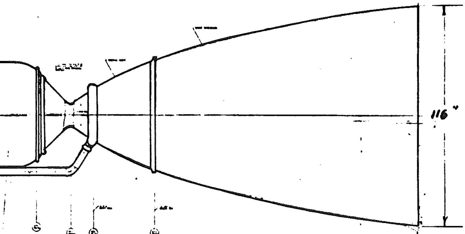
Figure 3 Rocket engine proposed by
'proposed by NASA' .Note the converging section, throat and diverging section.
Figure 3 shows a particular rocket motor proposed in the early 1970s. The addition of a diverging section then serves to achieve supersonic gas velocities. The narrowest part of the nozzle is termed "the throat", and the development of supersonic gas velocities coincides with maximum mass flow - choking - at the throat.
The nozzle must be designed for specified back pressure and specified reservoir pressure. Let us repeat a thought experiment employed for converging nozzles, by imagining various back pressures. Isentropic flows are possible only for some back pressures, and for other back pressures irreversible processes must occur. I present the isentropic pressure profiles only on Figure 4a and all pressure profiles on Figure 4b. The following observations hold (see Figure 4a).
\(p_{back} = p_o \) : the pressure is constant throughout the duct and gas is stationary;
\( p_o \gt p_{back} \gt p_{crit} \): the duct acts as a venturi. The greatest velocity is achieved at the throat - at no point does the gas achieve sonic velocity. The pressure decreases along converging section and then increases along the diverging section. The back pressure holds from the nozzle exit plane to the far field - some distance downstream of the exit plane;
\(p_{back}=p_{crit}\): the back pressure is equal to the critical pressure. At this stage gas achieves the speed of sound at the throat. The mass flow rate of gas can be increased no further and the nozzle is said to be choked . All other observations are as above;
\(p_{back} = p_{design} \): The nozzle is choked. The speed of sound is exceeded isentropically throughout the diverging section.
The above conditions 1-4 are amenable to analysis with the isentropic flow equations presented in the previous section. (Moreover, Equation 11 hints at the shape of the converging-diverging nozzle; for any scaled area (A/A*>1) two solutions exist with \( M \lt 1 \) and \(M \gt 1 \) ).
Figure 4b adds (in red) pressure profiles achieved irreversibly and away from the design point.
\( p_{design} \lt p_{back} \lt p_{crit}\): the supersonic flow undergoes a compression shock at a static shock wave . Pressure increases sharply. Thereafter flow is subsonic and isentropic.
Overexpanded nozzle with \(p_{exit}> p_{back}\):
The shock wave is at or very close to the exit plane and the nozzle is said to be overexpanded . The resulting overexpanded jet is
compressed outside the nozzle by a series of three dimensional, oblique shocks. The details are outside the scope of these notes. Note that the tendency of the back pressure to "squeeze" the jet detracts from the nozzle efficiency.
Underexpanded nozzle with \(p_{exit} \lt p_{back}\): A series of Prandtl-Meyer flow turns bring the flow pressure to the back pressure.
The above conditions feature irreversible processes that are not
amenable to analysis with the isentropic flow equations. The shock wave in condition 5 can sometimes be treated as a normal shock wave (see next section).
Figure 4 Pressure profiles along a converging-diverging nozzle (a) isentropic flows only (b) includes flows with shocks. See text for discussion of profiles 1, 2 ... 7.
Example CF0040 A reservoir holds air at pressure \(p_o= 10 bar \) and temperature \(T_o = 300K \).
A converging-diverging nozzle is to be designed to expand dry air isentropically
to a back pressure of 1.74 bar. Find the rate of mass flow through the nozzle and the thrust generated. The area of the throat is \(1.0 \times 10^{-4} m^2\)
Solution:
Problem statement: Find thrust and rate of mass flow through converging-diverging nozzle under design conditions.
Diagrams: See Figures 3 and 4, and in particular curve 4 in both parts of Figure 4..
Assumptions: Assumptions 1-6 in Section 4.2 above. For dry air \( \gamma = 1.4 = 7/5 \).
Physical laws: Mass conservation; energy conservation in form of SFEE, relating velocity and temperature changes; isentropic expansion, relating temperature and pressure.
Calculation:
Using the Ideal Gas Law the density and specific volume in the reservoir are \( \rho = 11.614 kg/m^3 \qquad v=0.0861 m^3/kg \). Look up \(p/p_o = 0.174 \) in column 2 of the isentropic flow table, Table 1, and find,
$$ p/p_o=0.174 \implies M=1.8 \qquad T/T_o = 0.6068 \qquad A/A^*= 1.4390 \qquad \rho/\rho_o=0.2868 $$
Then
$$ A_{exit}=1.0 \times 10^{-4} \times 1.4390 \qquad \rho_{exit} = 0.2868 \times 11.614 = 3.331 kg/m^{3} \qquad
T_{exit} = 0.6068 \times 300 = 182 K $$
The velocity in the exit plane is,
$$ c_{exit} = M_{exit} \sqrt {\gamma R T_{exit}} = 1.8 \times \sqrt {1.4 \times 0.287 \times 1000 \times 182 } = 487 m/s $$
$$ \dot{m}= A_{exit} c_{exit} \rho_{exit} = 1.439 \times 10^{-4} \times 487 \times 3.331 = 0.2334 kg/s $$
(Remember that rate of mass flow is constant throughout the nozzle. )
$$ Thrust = \dot{m} c_{exit} = 0.2334 \times 487 = 114 N $$
Alternative 1
The given problem aligned nicely with numbers in the flow tables (Table 1). Otherwise linear interpolation would be needed .(But I would suggest one uses tables with smaller steps in Mach number).Or one could
rearrange Equation 10 to obtain,
$$ \frac{p_o}{p}^{(\gamma-1)/\gamma} = (1 + M^2 (\gamma-1)/2) $$
$$ (10/1.74)^{2/7} = 1.6481 = (1+0.2 \times M^2) \implies M = 1.800 $$
Alternative 2
Mass flow rate could be found at the throat. If M=1 then \( \rho = 0.6339 \times 11.614 = 7.362 kg/m^3 \), \(T = 0.8333 \times 300 = 250 K \) and \( c= a = \sqrt{\gamma R T} = \sqrt{1.4 \times 0.287 \times 1000 \times 250} = 317 m/s\). The mass flow rate is
$$ \dot{m} = c A \rho = 317 \times 10^{-4} \times 7.362 = 0.2334 kg/s $$
This is particularly useful when investigators want to experiment with a range of back pressures.
Example CF0050 For the nozzle areas found in the above example CF0040, find the critical value of the back pressure
Solution:
The diagram, assumptions and physical principles are very similar to those in the previous problem CF0040, except refer to Curve 3 on Figure 4. For the back pressure defined in that example, \(A/A^*= 1.4390\). At the critical condition we have the same area, but the flow in the diverging section is subsonic, \(M \lt 1 \). Table 1 shows values on either side of the known area ratio,
The required solution is found by interpolation. (Tables with smaller increments of Mach number should be used for real world assessments. )
$$ x = (1.4390-1.5901)/(1.1882-1.5901) = 0.3760 $$
$$ M = 0.4 +0.2 \times x = 0.475$$
$$ p/p_o = 0.8956 + (0.7840-0.8956) \times x = 0.854$$
$$ p = 8.54 bar $$
Alternative 1: Experiment with the "Mach number of interest" box below the title for Table 1. A close match to the required area is
$$ M= 0.454 \implies A/A*= 1.4389 \; and \; p/p_o = 0.8682 \implies p=8.68 bar $$
The error in Mach number is about 4 per cent - one should use tables with
smaller increments of Mach number.
Alternative 2:
Substitute \( \gamma = 1.4 \; ; \; A/A* = 1.439 \) into equation 11 for A/A*. Then type ... "solve 1.439=(1/M)(5/6+(M^2)/6)^3"into Wolfram Alpha ( available at
https://www.wolframalpha.com/calculators/equation-solver-calculator/ ).
$$ M = 0.4540 \; or \; M= 1.80 $$
Recall that A* and \(A_{throat}\) are equal only when back pressure is less than or equal to the critical pressure. If the back pressure exceeds the critical pressure, \(A^* \ne A_{throat} \). A* will then need to be recomputed.
Example CF0060 Following on from CF0040 and CF0050, a converging-diverging nozzle operates subsonically with a reservoir pressure of 10 bar, a back pressure of 9.725 bar and an exit plane area \( A_{exit} = 1.439 A_{throat} \). Find the relationship between throat area and A*. Find the Mach number and pressure at the throat.
Solution:
The diagram, assumptions and physical principles are very similar to those in the previous problem CF0040, except refer to Curve 2 on Figure 4.
From table 1, at the exit plane
$$ p/p_o = 0.9725 \implies M=0.2 \; and \; A/A^* = 2.9635 $$
At the throat
$$ A_{exit}/A^* = 2.9635 \; and \; A_{exit}/A_{throat} = 1.439 \implies A_{throat}/A^* = 2.9635/1.439=2.059 $$
By trial and error (see "Mach number of interest in Table 1) I get to the point where \( A/A^*= 2.0590 \).
$$ M = 0.2961 \qquad p/p_o = 0.9410 \qquad A/A^*= 2.0590 \; (confirmed) $$
Then the pressure at the throat is 9.41 bar.
5. Shock Waves
When passing through a shock wave gas decelerates irreversibly, loses momentum and builds up pressure.
5.1 Normal shocks
The above discussion of a converging-diverging nozzle introduced the stationary normal shock wave (see Curve 5 on Figure 4). It is observed that:
the shock wave is thin (normally far thinner than any characteristic dimension of the nozzle);
the shock wave acts to pressurise any fluid passing through it - it is a compression shock ;
upstream flow is supersonic, downstream flow is subsonic.
In the analysis that follows, a set of assumptions apply.
flow is steady;
flow is one dimensional - there is no radial variation in velocity or pressure;
there is no transfer of work or heat between the surroundings and the flow;
ideal gas behaviour is often assumed (enabling use of \( pv = RT \) ).
I show the shock wave as N-S in Figure 5. A moving boundary (green) encloses a closed system: no mass passes the boundary. In part (a), at time \(t=0\), the leading edge of the moving boundary coincides with the shock. In part (b), at time \(t=\tau\), the moving boundary is sufficiently downstream for its trailing edge to coincide with the shock. The collapsible "detailed algebra" section below demonstrates the following principles.
Mass is conserved
$$ \frac{c_2}{c_1} = \frac {v_2}{v_1} \qquad \qquad (12) $$
where c is velocity, v is specific volume, 1 indicates the upstream state and 2 indicates the downstream state.
$$ h_o = h_1 + \frac{c_1^2}{2} = h_2 + \frac{c_2^2}{2} \qquad \qquad (6b) $$
where \( h_o\) is a quantity termed the "reservoir", "stagnation" or "total" enthalpy. It is the enthalpy the gas would have if it were brought isentropically to rest.
Entropy of a thermally isolated, closed system irreversibility can only increase
$$ s_2 \ge s_1 $$
Figure 5 Representation of a normal shock wave (NS). Red indicates lower pressure supersonic flow, blue indicates higher pressure subsonic flow. (a) time t=0, leading edge of (green) moving boundary is flush with normal shock wave and flow is supersonic (b) time t = tau, trailing edge of (green) moving boundary is flush with shock wave and flow is subsonic (c) pressure profile along duct (for all times).
I shall derive from first principles. Refer to Figure 5, where the imagined boundary of a closed system is shown by the green rectangles in parts (a) and (b). Let the respective conditions be 1 and 2. Then at 1 the length of the system is \(length = c_1 \tau \), the volume is \(V = length \times A = c_1 \tau A \), and the mass is \( m = c_1 \tau A / v \).
Mass conservation
Because the closed system mass is constant,
$$ m = \frac {c_1 \tau A}{v_1} = \frac {c_2 \tau A}{v_2} \qquad (A) $$
where m refers to the mass of the closed system (green rectangle) Area and time cancel so that
$$ \frac {c_1 }{v_1} = \frac {c_2 }{v_2} $$
Momentum conservation
The system decelerates from \(c_1\) to \(c_2\) subject to the restraining force \(A(p_2-p_1)\).
$$ A(p_2-p_1) = m \frac {c_1-c_2}{\tau} $$
Note in Equation (A) that system mass can be calculated from properties at station 1 or station 2. Substitute Equation (A) into the above,
$$ A(p_2-p_1) = \frac {c_1 \tau A}{v_1} \frac {c_1 }{\tau} - \frac {c_2 \tau A}{v_2} \frac { c_2}{\tau} $$
and if we cancel out A and \( \tau \),
$$ p_2 - p_1 = \frac{c_1^2}{v_1} - \frac{c_2^2}{v_2} \qquad \qquad (13) $$
5.2 Published ratios of temperature and pressure for a shock wave
For an ideal gas, the conservation equations in the previous section can be worked alongside the Ideal Gas Law and the Mach number definitions. The following expressions result (see collapsible section below) where 1 refers to the condition upstream of the shock and 2 refers to downstream. (Most text books quote ratios as a function of upstream Mach number only ( \(M_1\) ). The following equations demand less algebra and suffice to build Table 2.)
The temperature ratio (starting with energy conservation/ SFEE)
Consider the principles of energy, mass and momentum conservation in an ideal gas. Regardless of the reversibility of the flow, stagnation enthalpy ( and the stagnation temperature of an ideal gas) are constant across the shock (see Equation 6b above). In Equation 9 we substituted \(h= c_p T \) and the Mach number definition to relate static temperature to stagnation temperature.
$$ \frac{T}{T_o} = \frac{1}{1+ M^2( \gamma-1) /2 } \qquad (9) $$
work this with \(T \rightarrow T_1 \) and then \(T \rightarrow T_2 \) to get
Mass conservation gives an estimate of pressure ratio. Mass conservation satisfies,
$$ \frac{c_1}{c_2} = \frac {v_1}{v_2} \qquad \qquad (12) $$
Substitute the ideal gas law in the form
$$ \frac {v_1}{v_2} = \frac {T_1}{T_2} \frac {p_2}{p_1}$$
to obtain
$$ \frac{c_1}{c_2} =\frac {T_1}{T_2} \frac {p_2}{p_1}$$
To get an expression in terms of the dimensionless Mach number substitute Equation 4e, \( c_i = M_i \sqrt{\gamma R_i T_i } \) , into the above
$$ \frac{M_1}{M_2} \sqrt {\frac{T_1}{T_2}}=\frac {T_1}{T_2} \frac {p_2}{p_1}$$
Rearrange,
$$ \frac {p_2}{p_1} = \frac{M_1}{M_2} \sqrt {\frac{T_2}{T_1}} \qquad \qquad (14) $$
A second ratio of pressure can be found from momentum conservation,
$$ p_2 - p_1 = \frac{c_1^2}{v_1} - \frac{c_2^2}{v_2} \qquad \qquad (13) $$
For an ideal gas \(c_i^2 = M_i^2 \gamma p_i v_i \) so,
$$ p_2 - p_1 = M_1^2 \gamma p_1 - M_2^2 \gamma p_2 $$
Rearrange to obtain,
$$ \frac{p_2}{p_1} = \frac {1+ \gamma M_1^2 }{1+ \gamma M_2^2} \qquad \qquad (16) $$
Equations 14, 15 and 16 are combined to relate downstream and upstream Mach numbers.
Normal shock tables are published - Table 2 offers an illustrative example (the increments of Mach number are usually somewhat smaller).
Table 2 Calculator for normal shock waves: ratios of temperature, pressure and area versus Mach number.
Heat capacity ratio:
Gamma = :
Mach number of interest
M = :
To operate, input the Mach number of interest and heat capacity ratio in the boxes below and click "recalculate".
Results for the Mach number of interest are displayed in row 2 with a yellow background.
Example CF0070 Dry air has been accelerated to 1000 m/s, with Mach number \(M_1=3\). The air then undergoes a normal shock. Estimate the Mach number and velocity after the shock.
Solution:
Problem statement: Find the impact of a normal shock.
Diagrams: See Figure 5.
Assumptions: Assumptions 1-4 in Section 5.1 above.
Physical laws: To obtain tables - mass conservation; momentum conservation; energy conservation in form of SFEE . Thereupon, mass conservation or relation of velocity to Mach number and speed of sound.
Calculation:
From normal shock tables (or the applet in Table 2),
$$ M_1 = 3 \implies M_2 = 0.4752 \qquad \rho_2/ \rho_1 = 3.8571 $$
From mass conservation
$$ c_2/v_2 = c_1/v_1 \implies c_2 = \frac{c_1}{\rho_2/ \rho_1 } $$
$$ c_2 =\frac{1000}{3.8571} = 259 m /s $$
Alternatively,
$$ \frac{c_2}{c_1} = \frac{M_2 \sqrt{\gamma R T_2}}{M_1 \sqrt{\gamma R T_1}} = \frac {M_2}{M_1} \sqrt{T_2/T_1} $$
The temperature ratio is available from tables so,
$$ c_2 = 1000 \times \frac{0.4752}{3} \times \sqrt{2.6790} = 259 m/s $$
5.3 What entropy tells us about normal shocks
Whereas compression shocks are observed, rarefaction shocks are impossible.
Let us start with an equation for entropy change following a process with an ideal gas. (For the sake of generality, take the Gibbs Equation in Section 10 of the link, divide throughout by \(c_p\) and substitute Equation 8c above.)
Good books on Fluid Dynamics will demonstrate what happens when expressions for the temperature and pressure ratio are substituted into the above (e.g. Equations 14 to 17) so that entropy change is uniquely a function of \(M_1\) . The algebra is too fiddly for this note, but the important result is that entropy increases only for \(M_1 \gt 1 \). As the Mach number tends to unity entropy production tends to zero and one expects a reversible process. Because the nozzle is thermally isolated, the predicted decrease in entropy for lower Mach numbers is impossible according to the
8th corollary of the Second Law . Moreover, for \(M_1 \lt 1 \) specific volume is predicted to increase (density would decrease). This is known as rarefaction .
Consider the impact of irreversibility on the stagnation pressure, \(p_o\). Stagnation pressure would be constant for an isentropic process but the shock wave is anisentropic. Suppose gas starts in a gas reservoir 1, is accelerated isentropically, undergoes a shock, is decelerated isentropically to gas reservoir 2. Then the two gas reservoirs are at the same temperature - the stagnation temperature, and their pressures are equal to the stagnation pressures just upstream and just downstream of the shock wave. The above equation shows that, with reference to the states of the two gas reservoirs, increased entropy forces \(p_{o,2} \lt p_{o,1}\). (The logarithm of the ratio of stagnation temperatures is zero, and the logarithm of the ratio of stagnation pressures must be negative for entropy to increase.) That is, a shock must decrease stagnation pressure.
Another way to consider irreversibility would be to consider returning gas in gas reservoir 2 to gas reservoir 1, in such a way as to maintain the two reservoirs at a steady state. A return process that is theoretically possible requires isothermal compression from, \(p_{o,2}\) to \(p_{o,1}\), with the work input to the compressor equal to the heat output. Were one to claim falsely that \(p_{o,2} \gt p_{o,1}\), then theoretical steady state would be achieved by isothermal expansion, with a heat input and the equal amount of net power production transmitted to the surroundings. This corresponds to a cyclic engine receiving an amount of heat from a single reservoir and doing a net amount of work - it is impossible according to the
Kelvin-Plank statement of the Second Law of Thermodynamics . Furthermore, with regard to the stagnation pressure in Table 1 - \( \rho_2 \gt \rho_1 \) is evident only for rarefaction shocks with \(M_1 \lt 1 \; , \; \rho_2 \gt \rho_1 \).
Shocks reduce the isentropic efficiencies of nozzles, compressors and turbines. In turbo-machines, any shocks are often oblique. (See Section 5.4 below.)
Example CF0080 A reservoir holds dry air at 10 bar, 300K. The air is accelerated in a nozzle to M=2.4, at which point a shock occurs. (Thereafter air passes through a straight section, to mitigate effects of under-expansion.) Find the isentropic efficiency of the nozzle.
Solution:
Problem statement: Find the reduction in isentropic efficiency of a nozzle.
Diagrams: See Figure 4, curve 5.
Assumptions: Assumptions 1-6 in Section 4.2 above. Assumptions 1-4 in Section 5.1 above.
Physical laws: To obtain tables - mass conservation; momentum conservation; energy conservation in form of SFEE . Thereupon, mass conservation or relation of velocity to Mach number and speed of sound.
Physical laws:
I shall use subscript 0, 1, 2 to indicate respectively conditions in the reservoir, immediately
upstream of the shock and immediately downstream of the shock.
. Upstream of the shock \(A^*=A_{throat}\). From Table 1,
$$ M_1 = 2.4 \implies p_1/p_{o,1} = 0.0684 \qquad T_1/T_{o } = 0.4647 $$
From table 2 we obtain
$$ M_1= 2.4 \implies M_2= 0.5231\qquad p_2/p_1 = 6.5533 \qquad T_2/T_1 = 2.0403 $$
So the pressure just downstream of the shock is,
$$ p_2 = 6.5533 \times 0.0684 \times p_{o,1} = 0.442 p_{o,1} $$
where subscript o,1 refers to the upstream stagnation pressure. And the temperature is,
$$ T_2 = 2.0403 T_1 = 2.0403 \times 0.4647 \times T_{o } = 0.9481 T_{o} $$
(Remember that stagnation temperature is constant and there is no need to distinguish between upstream and downstream values.)
Let us consider an alternative, isentropic process from reservoir pressure (10 bar) to \(p_2\). The end temperature would be,
$$ T_{2,isen} = T_o (\frac{p_o}{p_2})^{(\gamma-1)/\gamma } = 0.422^{2/7} T_o = 0.7815 T_o $$
And the isentropic efficiency is,
$$ \eta_{isen} = \frac{T_o-T_2}{T_o-T_{2,isen}} = \frac {1-0.9481}{1-0.7815} = 23.8\% $$
5.4 Oblique shocks
A shock wave can lie obliquely to the direction of flow.
This is well known in supersonic flight .
Principles are:
The velocity is resolved into components normal to the shock wave and tangential to the shock wave;
the tangential velocity component is treated equal on both sides of the shock wave;
property changes are found from the normal shock relations, using with the normal component of upstream velocity or Mach number.
In addition to the assumptions list for Section 5.1, one adds the assumption of equal tangential components of velocity .
Figure 6 shows a shock wave (in red) inclined at the shock angle \( \theta \) to the upstream direction of flow. The shock deflects fluid through a deflection angle \(delta\). Although the deflection angle is the easiest to specify - e.g. from the geometry of a wedge - it is easier to calculate it as a function of \( \theta \), possibly as part of a trial and error approach.
Let us apply principles of mass conservation to the normal velocity components.
$$ c_{2n} = \frac{c_{1n}}{ \rho_2 / \rho_1 } $$
and the density ratio is computed using \(M_{1n}\), the normal component of upstream Mach number. Trigonometric analysis yields,
$$ \delta = \theta - atan \frac{c_{2n}}{c_t} $$
Substitute for \(c_{2n}\) in the above,
$$ \delta = \theta - atan \frac{c_{1n}}{c_t \rho_2 / \rho_1 } \frac{ }{} $$
a bit more trigonometry tells us that \(tan \theta = \frac{c_{1n}}{c_t} \) and hence
$$ \delta = \theta - atan (tan \theta / \frac{\rho_{2}}{\rho_{1}} ) $$
The above suffices for problem solving. With some difficult algebra, functions are usually expressed principally in terms of upstream Mach number, see for example the NASA web pages .
Figure 6 An oblique shock (red) showing tangential and normal components of velocity upstream and downstream of the shock. The shock is inclined at angle \(beta\) to flow direction, and flow is deflected by angle \(delta\).
Example CF0090
A projectile moves through still air in a straight line Mach number \(M_1 = 2.309\). The shock wave thus formed is at 60 degrees to the flight path. Relative to the projectile, find the Mach number and angle of deflection downstream of the shock.
Solution:
Problem statement: Find the impact of a normal shock.
Diagrams: See Figure 6.
Assumptions: Assumptions 1-4 in Section 5.1 above. There is no change in tangential components of velocity, and properties are determined from the normal component of upstream Mach number;
Physical laws: To obtain normal shock tables - mass conservation; momentum conservation; energy conservation in form of SFEE . Thereupon, mass conservation or relation of velocity to Mach number and speed of sound.
Calculation:
Downstream of the shock, use the lengths of a bisected isosceles triangle to find components of Mach number,
$$ M_{1n} = 2.309 \times \times \sqrt{3}/2 = 2 $$
Feed M=2 into normal shock tables to obtain,
$$ M_{2n} = 0.5774 \qquad \qquad \qquad \rho_2/\rho_1 = 2.6667 $$
$$ \delta = \theta - atan (tan \theta / \frac{\rho_{2}}{\rho_{1}} ) =60^o - atan (\frac{tan 60^o}{2.6667}) = 60-33=27^o$$
$$ M_2 = M_{2n}/sin(\theta-\delta) = 0.5774/sin(60^o-27^o) = 1.06$$
Note that if the upstream velocity were specified we could look up the temperature ratio and use it to obtain downstream velocity,
$$ \frac{c_2}{c_1} = \frac{M_2 \sqrt{\gamma R T_2}}{M_1 \sqrt{ \gamma R T_1 }} = \frac{M_2}{M_1} \sqrt{T_2/T_1}= \frac{1.06}{2} \sqrt{ 1.6875}
= 0.6885 $$
For an oblique shock to happen, the normal component of Mach number must exceed one (rather than its absolute value). On the other hand, suppose that, after an oblique shock, the vector addition of tangential and normal components exceeds one. Then a further, second shock is possible upon further changes in the flow direction. That is, multiple oblique shocks are possible.
The mathematical solution is explicit for the angle of flow deviation but implicit for the shock angle. The frequent requirement for the shock angle necessitates iterative solution. Alternatively, one can refer to tables such as
in NACA TN No. 1673 .