These notes concern principally the sizing of refrigerators and heat pumps. The reader is assumed to have studied previously the following topics:
the First Law of Thermodynamics and the Steady Flow Energy equation;
steam cycles - in particular the use of tables to deal with non-ideal fluids.
We offer two types of process map - Ts diagrams and ph (pressure enthalpy) diagrams. Processes on both maps can be
studied with our
interactive chart. The refrigerant is ammonia.
2. Introduction
When the applied pressure is reduced sufficiently, a liquid will boil at below room temperature and absorb heat from its surroundings.
Vapour compression cycles are employed in refrigerators and heat pumps.
Refrigeration is used in air conditioning and for the storage of food and other heat sensitive products.
Heat pumps are now an important part of the debate concerning low-carbon space heating.
Rather crudely, refrigeration cycles can be envisaged as the reverse of steam power cycles.
Many types of refrigerant are available - this topic concerns the cycle thermodynamics far more
than the chemistry and selection of refrigerants.
It is intended that the reader will be able to:
draw plant diagrams for three types of cycle;
represent cyclic processes on a T-s diagram and/or on a p-h diagram;
identify separate processes within refrigeration, particulaly those with constant h, p, s, T;
carry out energy balances over plant items;
compute the coefficients of performance of three types of refrigerator;
be aware of alternatives to vapour compression.
A historical perspective is instructive.
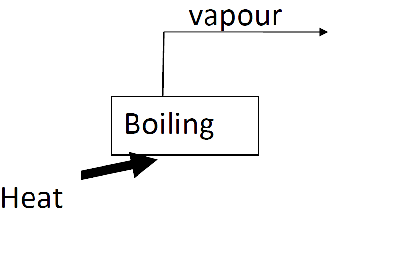
In 1745 William Cullen caused ether to boil and thus cool by application of a vacuum. His makeshift evaporator absorbed heat in order that the ether might change phase, from liquid to vapour, at room
temperature or less. This demonstration suffered two limitations (1) obviously, the evaporator would eventually boil dry (2) only atmospheric pressure can apply at the exit from the vacuum pump (cum compressor). Thus the pressure ratio of the compressor is fixed and the power input might be excessive (high pressure ratio) or the ``temperature lift'', in terms of ambient temperature minus evaporator temperature, might be too small (low pressure ratio).
Vapour compression cycles are the most widely used. The cycle exploits the strong influence of pressure on boiling point; hence the evaporator absorbs heat at a lower temperature and pressure and the condenser rejects heat at a higher temperature and pressure.
The study of refrigeration covers many plant items previously seen - heat exchangers, turbines, compressors, throttles (and even combustion). Refrigeration applies to food storage, heating ventilation and air conditioning (or HVAC), heat pumps and total energy schemes.
Most of this series will cover the vapour compression cycle. This is the most common form of refrigeration, but it is worth noting that other forms exist.
If we start with the simplest idea (William Cullen's) cooling would follow if a liquid (= refrigerant) was evaporated at a pressure below atmospheric pressure. This idea has two limitations (1) the evaporator would eventually boil dry (2) the pressure ratio is fixed by the boiling temperature of the refrigerant (in turn fixing the boiling pressure) and the exit pressure of the required vaccuum pump - 1 atm approx. There is no guarantee that the pressure ratio is optimum.
Figure 1 William Cullen's demonstration
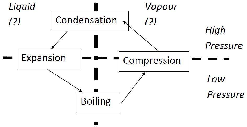
Continuous operation is achieved through a cycle. The cycle exploits the (approximately exponential) variation of vapour pressure with temperature. Thus by changing pressure the same liquid can be forced to boil at a lower temperature (~4oC) and lower pressure and condense at a higher temperature (~30oC) and higher pressure
Figure 2 Representation of a vapour cycle (My own idea, not in textbooks)
3. Refrigerant Behaviour and Properties
The enthalpy, entropy and saturation pressure of commonly used refrigerants are tabulated.
In principle any liquid can act as a refrigerant - that is at low pressure it has a comparatively low boiling point and at high pressure it has a comparatively high condensation temperature. The first commercial refrigerants included ammonia (R717) and the alkanes. These were (respectively) toxic and flammable, but are back in use owing to the ozone depletion potential and global warming potential of the chlorinated fluoro carbons. Rogers and Mayhew tablulate data for ammonia, dichlordifluoromethane (R12), and tetrafluoroethane (R134a). (R12 is now illegal and R134a is in the process of being phased out.)
Example uz010: Find the properties of R717 at 4.295 bar.
Obtain (1) the saturation temperature (2) the specific enthalpy of saturated liquid for this pressure (3) the corresponding specific enthalpy of saturated vapour (4) the specific enthalpy of vapour at 30oC.
(1) Column 1 gives
\(T_s=0^oC\)
(2,3) Columns 4 and 5 give
\(h_f=181.2kJ/kg\)
and \(h_g=1444.4 kJ/kg\) (4) Column 8 gives the enthalpy at \((T – T_s) = 50 K\) or \(T = T_s + 50 K = 0 + 50 = 50^oC\). The given value is 30K hotter than Ts. Noting that \(30K/50K = 0.6\) we find the specific enthalpy requested is \(0.4 \times 1444 + 0.6 \times 1568=1518 kJ/kg\).
You can check the above at
our interactive Ts chart . Along the part of the isobar between saturated liquid (f) and saturated vapour (g) the temperature is the saturation temperature, 273.15K. The plotter produced the enthalpies at points 2,3, 4 broadly in line with the above estimates, subject to manual errors. (Should you want to obtain more precise estimates, use numerical entry rather than mouse clicks. Note that precise data are unavailable in the white region.)
Example uz020: For R717, how hot would saturated vapour at \(0^oC\) become if compressed reversibly to 8.570 bar.
Solution: Let vapour enter the compressor at 1 and leave at 2. The isentropic compression means that the exit entropy is \(s_2=s_1 =5.340 kJ/kgK\ \). Locate the pressure p=8.57 bar in column 2. Column 1 gives the saturation temperature, \( T_s = 20^oC \), but this is not the true temperature because at saturation the entropy is less than required, \( s_g=5.095<5.34kJ/kgK \). Column 9 refers to the entropy that superheated vapour would have with a degree of superheat of \(T-T_s=50K\) ; \(s = 5.521 kJ/kgK \) which exceeds the required value. Interpolation between columns 7 and 9 gives
\( T - T_s = 28.8 K \) and therefore \(T = 20 + 28.8 = 48.8^oC \).
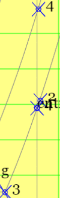
Using the online plotter, I get a temperature of 47.0oC (320.2K), subject to plotting errors. See symbol 2 on the plot below.
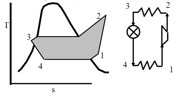
4. The Reversed Carnot Cycle
The Reversed Carnot Cycle illustrates several aspects of refrigeration:
compression, expansion, evaporation, condensation, evaporation, wet vapour.
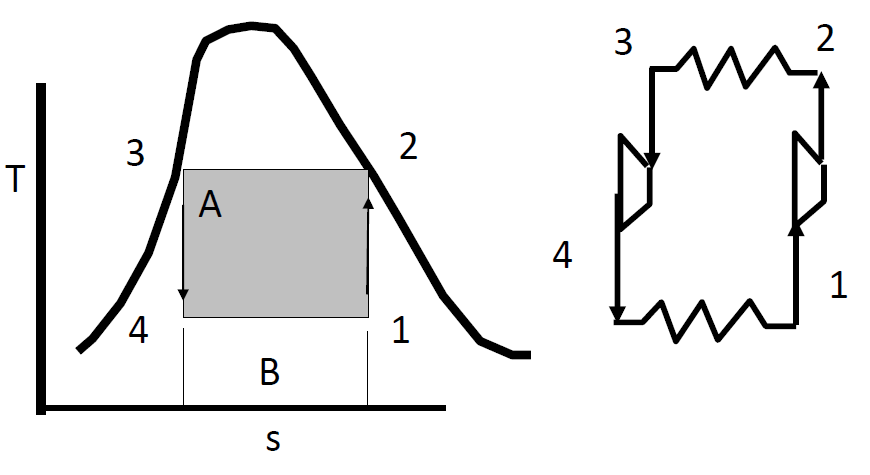
The simplest cycle is the reversed Carnot cycle. (This is not a practical cycle, for reasons that will be explained shortly). On a cycle diagram, the path looks very similar to that introduced earlier for pure gases. The difference is that the path lies underneath the saturation lines for liquid (f) and vapour (g) on the T-s diagram. Anything underneath this envelope is wet vapour - a two phase mixture of liquid and vapour (typically droplets plus vapour). The left hand side of the envelope traces saturated liquid (f). The right hand side of the envelope traces saturated vapour (g).
Figure 3 Basic Carnot cycle, including vapour compression.
The four processes are:
1-to-2: Isentropic compression, wet vapour enters the compressor at (1), high pressure saturated vapour leaves at 2. Work is added to the system
2-to-3: Condensation, the state of refrigerant changes from saturated vapour (2) to saturated liquid (3). The heat of vaporisation is released to the environment.
3-to-4: Isentropic expansion, starting with saturated vapour at (3) and finishing with wet vapour at (4). For the isentropic process this is effected by a turbine, so that work is recovered and the net work demanded is \( |W_{comp}|-|W_{turb}|\).
4-to-1: From the diagram, one notes that point 4 is closer to the saturated liquid line (f) than point 1 - it is wetter. From 4-to-1 some liquid is evaporated, achieving the higher dryness fraction at 1. Heat addition is necessary, that is heat is absorbed from the environment.
Because this is a reversible process, the net work input (= compressor work minus turbine work) is area 1-2-3-4 and the heat absorbed is area under 1-4 (as was the case in year 1). We can define coefficient of refrigeration as the cooling power per unit net work and
\begin{equation}
COP = \frac{q_{41}}{|w_{12}+w_{34}|} = \frac{T_{14}}{T_{23}-T_{14}}
\end{equation}
Example uz030: Find the COP of a Carnot cycle refrigerator operating with ammonia as a refrigerant. Take temperatures as 20oC in the condenser and 0oC in the evaporator.
Solution: See Figure 3. Assume isentropic expansion and compression.
Tables give saturation properties relevant to the condenser:
Noting that in the evaporator \(s_1=s_2 \; and \; s_4=s_3 \) the dryness fractions follow from the wet property relationships ,
\begin{align*}
x_1 &= (5.095-0.715)/(5.340-0.715) = 0.9470 \\
x_4 & =(1.044-0.715)/(5.340-0.715) = 0.0711 \\
h_1 &= 181 + 0.9470 \times (1444-181) = 1377 kJ/kg \\
h_4 &= 181 + 0.0711 \times (1444-181) = 271 kJ/kg
\end{align*}
The specific work for the compressor and turbine follow from the SFEE; KE and PE changes are ignored. The heat transfer from the evaporator similarly follows.
\begin{align*}
w_{12} &= h_2-h_1 = 86 kJ/kg \\
w_{34} &= h_4-h_3 = -4 kJ/kg \\
q_{41} &= h_1-h_4 = 1106 kJ/kg
\end{align*}
The coefficient of performance (for refrigeration) is then the absorbed heat transfer per unit net work input
The above is provided for the purposes of illustration only. Taking all processes as reversible we ought to obtain the same result from Equation 1 using temperatures only. Indeed COP = 273/20 = 13.65 which (allowing for rounding errors) is identical to the more laborious estimate.
As a further check, the corresponding energy flows from the plotter are,
$$ COP = \frac {-1117}{81.5-5.9} = 14.8 $$
which (allowing for plotting errors) is very broadly in line with the previous estimates.
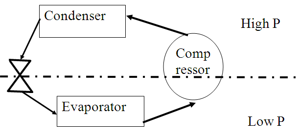
5. Simple Practical Systems
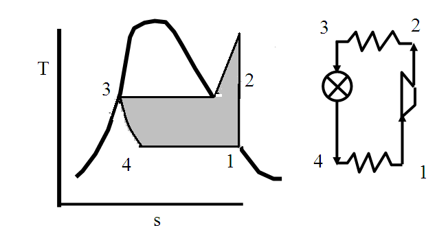
For practical reasons, in a basic cycle fluid is expanded isenthalpically (with constant enthalpy) and irreversibly.
Even if reversible processes were realisable wet vapour cannot be passed through expanders and compressors (or at least not for a long period of time). Thus in the simplest tutorial question regarding a practical system one finds the following.
the turbine is replaced with a throttle (= valve almost closed)
the throttle acts isenthalpically. That is, \(h_3 = h_4\)
the compressor intake is in the form of saturated vapour (g).
One might query the assumption of isenthalpic operation in the throttle. The production of vapour increases specific volume and therefore velocity and kinetic energy, at the expense of enthalpy. This energy conversion is very small compared to energy transfers elsewhere.
Figure 4 Idealised representation of a practical cycle.
However, we note in a more realistic system (1) the compressor acts irreversibly (2) any change in heat load could reduce the specific enthalpy of the evaporator outlet, changing the condition from saturated vapour (g) to wet vapour. As a safety factor, the evaporator exit is often slightly superheated. (3) Condenser design is not a precise science, and typically 20% overdesign is recommended. The compressor exit is likely to be subcooled (that is, at a temperature less than the saturation temperature for the associated pressure).
Figure 5 A more realistic representation of the practical cycle
Energy Balances
In the SFEE, we ignore changes in kinetic and potential energy. Thereafter the
throttle is not designed to develop work, and is too small to transport appreciable amounts of heat. The operation of the throttle is isenthalpic , that is
\begin{equation}
\dot{Q}_{34}=\dot{W}_{34}=0= \dot{m}(h_4-h_3) \implies h_3=h_4 \qquad throttle
\end{equation}
\begin{equation}
\dot{Q}_{14}=\dot{m}(h_1-h_4)=\dot{m}(h_1-h_3) \qquad evaporator
\end{equation}
The isenthalpic expansion across the throttle explaims \(h_3 = h_4\).
For a refrigerator (as opposed to a heat pump) the coefficient of performance is the amount of heat adsorbed by
the evaporator per unit of work input to the compressor.
\begin{equation}
COP = \frac{\dot{Q}_{41}}{\dot{W}_{12}}
\end{equation}
Recall that refrigerant properties are tabulated in
'Steam tables' .
Example uz040: for R717 Find the COP of a basic practical refrigeration cycle operating between saturation temperatures of \(0^oC\) and \(20^oC\).
Solution:
Assume that ammonia is the working fluid, that compression is reversible (isentropic) so that \(s_1=s_2\), that fluid leaves the evaporator and condenser in saturated condition. Refer to Figure 4 for plant diagram.
The enthalpy at 1 was calculated previously as \(h_1= h_g = 1444 kJ/kg\). At 2 \(s_2=s_1=5.340 kJ/kgK\)(reversible, isentropic compression) and by interpolation \(h_2 = 1463+(340-95)\times(1597-1463)/(521-95) = 1\;540kJ/kgK\). Note the isenthalpic throttle so \(h_4=h_3=h_f=275kJ/kg\).
The COP is the heat absorbed in the evaporator per unit work done on the compressor. For isentropic conditions
\begin{equation*}
COP = \frac{q_{41}}{w_{12}}= \frac{h_1- h_3}{h_2-h_1} = 12.1 \qquad note \; h_3 = h_4
\end{equation*}
As a rough check, the online plotter gives corresponding heat flows as
$$ COP = \frac{1170}{93} = 12.6 $$
(Note the 'change row'. Clicking on the chart in the sequence 4-1-2 yields the enthalpy changes from 4-1 and 1-2.)
This is higher than typical refrigerator COPs, not unusually quoted as in the region of 2.0 to 3.0. The domestic compressor will have a low isentropic efficiency (seldom
quoted, but I have seen values in the range from 0.4 to 0.7). The evaporator should be somewhat colder than the load to enable heat transfer, and likewise the condenser
should be hotter than its surroundings. For example with evaporator temperature 263K, condenser temperature 303K, and an isentropic efficiency of 60% the online check gives
me COP = 3.4. In addition the domestic unit's larger ratio of surface area-to-volume can promote an appreciable heat loss - the SFEE should be modified appropriately.
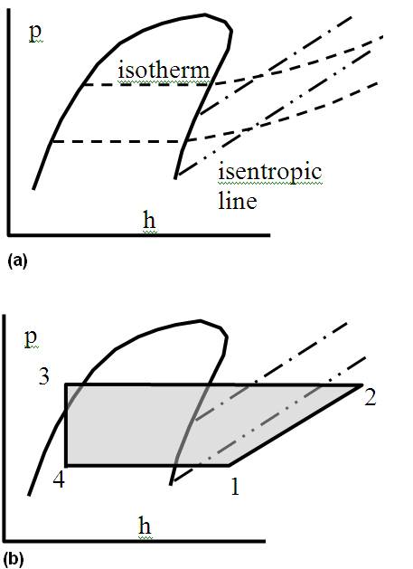
Pressure Enthalpy Diagrams
In addition to temperature versus entropy, refrigeration engineers often represent the cycle on plots of pressure-vs-specific enthalpy, p-h diagrams. Specialist graph paper comes with p-h marked on the y-x axes, and with lines of constant temperature (isotherms) and constant entropy (isentropic lines). The saturation states (f and g) are also represented. One benefit is that it is easy to visualise the coefficient of performance. In the diagram horizontal length 1-to-4 is in proportion to the cooling effect and horizontal length 1-to-2 is in proportion to the compressor power.
Figure 6 The p-h Diagram (a) with isentropic line and isotherm (b) full practical cycle
Example uz050: for R717 find the COP of a basic practical refrigeration cycle operating between saturation temperatures of 263.15K and 298.15K, with
compressor isentropic efficiencies of 100% and 75%.
Solution: I used the
online plotter to produce the figure below. Paper charts are populated with families of isotherms and constant entropy lines; at the required conditions isentropic and isothermal curves should be interpolated. The steps in analysis were:
Use keyboard input to select T=268.15K, dryness =1 .
Set the above as point 1 and plot an isobar through it (red).
Similarly select T=298.15K, dryness = 0 as point 3. Plot an isobar through it (red).
Plot a curve of constant entropy (green) through point 1. Mark symbol 2 where this passes through the upper isobar.
Plot a vertical line of constant enthalpy through point 3, mark symbol 4 where this passes through the lower isobar
Measure the enthalpy changes from 1-to-2 (compressor) and 3-to-1 (same as 4-to-1 evaporator).
From the measured enthalpy changes,
$$ COP = \frac{|q_{41}|}{w_{12}} = \frac{h_3-h_1}{h_2-h_1} \approx \frac{1130}{177} = 6.4 \qquad; isenthalpic \; expansion \; \implies \; h_4 = h_3 $$
Adjust the denominator in order to deal with isentropic efficiency. Thus
$$ COP = \frac{|q_{41}|}{w_{12} / 0.75} = 6.4 \times 0.75 = 4.8 \qquad anisentropic \; compression $$
Example uz055: A simple practical cycle employs ammonia (R717) as its working fluid. The saturation temperatures are \(-4^oC\)in the evaporator and \(34^oC\) in the condenser. Refrigerant leaving the evaporator is superheated by 5K. Refrigerant leaving the condenser is subcooled by 4K. The compressor acts irreversibly with an isentropic efficiency of \(\eta_{isen}=45\%\). Find the refrigerator's coefficient of performance.
Solution: I shall use the pressure-enthalpy plot on the
interactive Ts chart . At the saturation temperature of \(-4^oC = 269.15 K \) the corresponding
pressure at saturation is 3.662 bar and along this isobar, at \(T_1 =-4+5^oC = 274.15K \),
$$ h_1 = 1453.1 kJ/kg \qquad s_1 = 5.445 kJ/kg K $$
(nb, steam tables give s1=5.433kJ/kgK). For \(34^oC\) the saturation pressure is 13.031 bar, and at this pressure, \(30^oC\)
$$ h_3 = h_4 = 322.7 kJ/kg $$
(NB, keyboard entry is needed to plot a point in the subcooled region.) The isentropic line and higher isobar intersect at
point 2', where,
$$ h_2' = 1641.7 kJ/kg $$
Take differences in enthalpy to get,
$$ q_{14} = 1130.4 kJ/kg \qquad w'_{12} = -188.6 kJ/kg$$
$$ COP_{isen} = 1130.4/188.6 = 5.99$$
$$ COP = 7.05 \times 0.45 = 2.7$$
Note that the anisentropic line is off scale.
As a check, measure enthalpy changes on the chart (click on the sequence 4-1-2 and read enthalpy in the "change" row)
$$ q_{14} = 1133.4 kJ/kg \qquad w'_{12} = -186.8 kJ/kg $$
This gives the same COP (to 2 s.f.s).
Figure showing imperfect practical cycle. I have drawn isobars in red, isentropic curves in blue,
and the isenthalpic line in green.
Heat Pumps
The heat pump operates in exactly the same way as the refrigerator. The difference is in the
purpose, which is to extract heat from the environment and "upgrade" it for heating purposes. Thus, rather than the heat absorbed by the evaporator the engineer is concerned with the heat rejected from the condenser. Heat pumps are advertised as energy efficient - typically 1 joule of mechanical power yields 4 joules of heating effect.
\begin{equation}
COP_{HP}= |\frac{\dot{Q}_{23}}{\dot{W}}|= 1+|\frac{\dot{Q}_{41}}{\dot{W}}|
\end{equation}
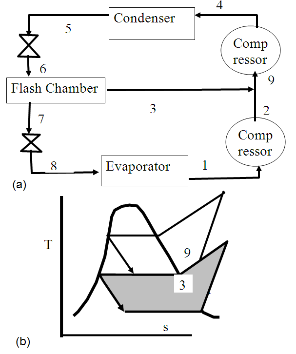
6. Multistage Compression
For very large temperature lifts, more elaborate plant is
used to retain a reasonable load on individual compressors and achieve an acceptable coefficient of performance.
The simpler practical cycles work well for uses such as chilling food (\(4^oC\)) and adequately for freezing it (\(-18^oC\)). But at lower temperatures refrigerant exiting the expansion valve is too dry - the anisentropic expansion "moves" refrigerant away from the saturated liquid (f) curve and toward the saturated vapour (g) curve. Colder temperatures force less cooling per unit mass of refrigerant and greater power demand for compression - the net effect is a reduced coefficient of performance. A further problem is that lower temperature results in a reduced pressure and thereupon a bigger compressor ratio.
Figure 7 Basic Cycle.
A further way of looking at this is to consider what happens when refrigerant enters the evaporator with a big dryness fraction. For every 1 kg of refrigerant we have x kg of vapour and this first passes through the evaporator absorbing zero or minimum heat but then demands word from the compressor.
Two strategies are possible; this section discusses multistage compression . Multistage compression
operates at three pressures (rather than two).
On the right hand side of the plant, vapour pressure is increased from low-to-intermediate-to-high with two compressors in series. Stream 3 will be discussed shortly, but note that fluids in streams 3 and 2 are mixed to give stream 9, the inlet to the high-pressure compressor.
On the left hand side of the plant expansion is achieved in two stages. At 6 wet vapour enters a flash chamber at intermediate pressure. The flash chamber is simply a vessel, arranged so that the wet vapour stratifies into separate layers of liquid and vapour. We assume refrigerant exits in these two forms: saturated vapour (stream 3) and saturated liquid (stream 7). Note that all streams entering and leaving the chamber (6, 3, 7) have the same (intermediate) pressure.
Thus, the flash chamber removes some vapour that would otherwise have had minimal refrigerant effect within a cycle, but would
require the processing of two compressors - this vapour must now be processed by one
compressor only.
Let us now consider analysis . The treatment of compression and isenthalpic expansion are identical to those explained in the topic on basic cycles. The new calculations apply to the flash chamber and the mixing point; both operate at the intermediate pressure. Combining the flash chamber and high pressure throttle (isenthalpic expansion, \(h_5=h_6\)), let us draw a boundary cutting the streams of saturated fluid: 5, 3 and 7. The three enthalpies are available in tables. The energy balance yields the dryness fraction in stream 6 and the mass flow of vapour in stream 3, \( \dot{m}_3 = x_6 \dot{m}_5 \). Take a basis of 1 unit mass of refrigerant in streams 5 and 6.
\begin{equation}
h_5=h_6= x_6 h_3 + (1-x_6) h_7 \qquad \implies x_6
\end{equation}
On the assumption of adiabatic mixing at the mixing point.
\begin{equation}
h_9 = x_6 h_3 + (1-x_6)h_2
\end{equation}
This is the enthalpy of superheated vapour fed to the HP compressor.
Three flow rates are at play. Let us normalise flows by setting a basis of
1 unit mass in streams 9,4, 5, 6. The flow in stream 3 is then \(x_6\) . The
flow in streams 7, 8, 1, 2 is (\1-x_6\) . For convenience, I shall omit
subscript 6 from this point
The COP is computed from heat addition to the evaporator and work addition to the two compressors. Be alert to the second compressor dealing with a greater flow of mass than the two other components. Taking the mass flow rate through the condenser, \(\dot{m}_4\), one obtains the rates of energy transfer.
\begin{align*}
\dot{W}_{12} &= \dot{m}_4 (1-x)(h_2-h_1) \\
\dot{W}_{94} &= \dot{m}_4 (h_4-h_9) \\
\dot{Q}_{81} &= \dot{m}_4 (1-x) (h_1- \, h_7) \qquad nb \; h_7 = h_8 \\
\end{align*}
And the coefficient of performance is
\begin{equation}
COP_{ms} = \frac{\dot{Q}_{81}}{\dot{W}_{12}+\dot{W}_{94}}
\end{equation}
Substitute the enthalpies to botain,
\begin{equation}
COP_{ms} = \frac{(1-x) (h_1- h_7) }{(1-x)(h_2-h_1)+(h_4-h_9)}
\end{equation}
Point out in example that two intermediate pressures are identical.
Example uz060: Find the coefficient of performance of a multistage compression cycle with ammonia pressures of 1.196, 4.295 and 8.570 bar.
2. Find the ethalpy at the LP compressor exit (use online plotter or see example uz040). Carry out SFEE over the flash chamber and find the dryness fraction.
See Figure b.
$$ h_2 = 1576 kJ/kg \qquad subject \; to \; plotting \; error $$
$$ h_5 = x h_3 + (1-x) h_7 \qquad rewrite \; x_6 \; as x $$
$$ 275.2 = x \times 1445.5 + (1-x) \times 181.0 = 181.0 + 1264.5 x $$
$$ x = (275.2 - 181.0) / 1264.5 = 7.45\% \qquad (vs \; 7.7\% \; by \; interactve \; plotter ) $$
(The interactive plotter will be subject to manual error).
3. Carry out SFEE at the mixing point - 2,3,9 - to get h9 (HP compressor input). Find the compressor exit enthalpy (use
online plotter or see example uz040).
Hint - point 9 is very close to point 2. I zoom in below. Points
3,9,2 lie in that sequence along the isobaric curve, and the vertical isentropic line
extends from point 9 to point 4.
(Compare this with a previous estimate of 4.14, using
'Steam tables'
and finding compressor exit conditions at 2 and 9 by linear interporation,
rather than online plotter)
7. Cascade Refrigeration
The efficiency of the multistage process can be achieved in a different way that (in principle)
allows two different refrigerants to be used for the two different pressure ranges. This comes at
the expense of an additional heat exchanger. If effect, two refrigeration cycles are employed to pump heat from low-to-intermediate-to-high temperature.
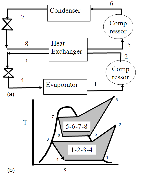
Figure 9 Cascade refrigeration (a) plant diagram (b) T-s diagram. The separation of (8,5) and (2,3) is artistic license. In many text book problems the two sets
share the same saturation temperature (T3 = T8) whereas for practical purposes heat
transfer demands that \(T_3 > T_8\).
Note the "topping cycle" (intermediate and high pressure) and "bottoming cycle" (intermediate and low pressure). The heat exchanger provides condensation for the bottoming cycle (streams 2 and 3) and evaporation for the topping cycle (streams 5 and 8). The nub of the problem solving methods is to note that under certain assumptions the heat rejection from the bottoming cycle equals the heat addition to the topping cycle.
\begin{align*}
(-1) \times\dot{Q}_{23} & = \dot{Q}_{58} \implies \\
\dot{m}_b(h_2-h_3) & = \dot{m}_t(h_5-h_8) \\
\end{align*}
Standard assumptions are: steady conditions, constant pressure from 2-to-3 and 5-to-8, no extraneous heat loss/ gain, ignore changes in potential and kinetic energy. In worked examples in text books, it is common to see identical intermediate pressures used, that is \( p_2=p_3=p_5=p_8\). (In fact saturation temperature \(T_3\) must exceed saturation temperature \(T_5 = T_8\) to drive heat transfer. This contradicts artistic license in the above T-s diagram.)
The processes of compression, isenthalpic expansion and evaporation are identical to those described in the
section on practical cycles.
A typical problem might be solved as follows. The two intermediate pressures might be treated as equal.
Thus the system is specified by three isobars that include the three sequences of points 4-1, 3-8-5-2, and 7-8. The above energy balance yields the ratio of mass flows in the topping and bottoming cycles upon which work transfer to the two compressors and heat transfer to the evaporator are computed.
\begin{align*}
\dot{Q}_{14} & = \dot{m}_b (h_1-h_3) \\
\dot{W}_{12} & = \dot{m}_b(h_2-h_1) \\
\dot{W}_{56} & = \dot{m}_t(h_6-h_5) \\
COP_{cas} &= \frac {\dot{Q}_{14}} {\dot{W}_{12} + \dot{W}_{56}} = \frac{h_1-h_3}{h_2-h_1 + (\dot{m}_t/\dot{m}_b)(h_6-h_5)}
\end{align*}
Example uz070: Find the COP of a cascade cycle with ammonia pressures of 1.196, 4.295, 4.295 and 8.570 bar. Refrigerant emerges from HP compressor with 50 K superheat
Solution:
See diagrams in notes. Assume reversible compression (at lower pressure), no superheat at evaporator exit, no sub-cooling at condenser exit, steady operating conditions, isenthalpic expansion. Implicit in the specified pressures is that there is no temperature difference in the intermediate heat exchanger.
The enthalpies of saturated fluids were found in the previous example. Some serial numbers are changed.
$$ h_1 = 1404.2 kJ/kg \qquad h_3= 181.0 kJ/kg \qquad h_5 = 1445.5 kJ/kg \qquad h_7= 275.2 kJ/kg \qquad \qquad $$
Also found previously $$ h_2 = 1576 kJ/kg \qquad subject \; to \; plotting \; error $$
Regarding the HP compressor, at 8.570 bar the saturation temperature is \(T_{sat}=293.4 K \) (this is from my online plotter - tables give a slightly different value of 293.15K).
Then \(T_6= 343.4K \) and at 8.570 bar, 343.4K ,
$$ h_6 = 1596.9 kJ/kg $$
The eight states and isobars are plotted here. I show isenthalpic curves in red
Use the energy balance to get the ratios of flow in the topping and bottoming cycles.
$$ \dot{m}_b( h_2-h_3) = \dot{m}_t (h_5-h_8) \qquad nb \; h_7 = h_8 $$
$$ m_t = m_b \frac {h_2-h_3}{h_5-h_7} = m_b \frac {1576-181}{1445.5-275.2} = m_b \frac {1395}{1169} =1.193 $$
Then find the coefficient of performance.
$$ COP = \frac{\dot{Q}_{41}}{\dot{W}_{12} + \dot{W}_{56} } = 3.47 $$
Appendix - Miscellaneous Processes
Here are some non-standard cycles. In addition to coefficient of performance, we want to select cycles on basis of utility, environmental impact, reliability of supply/ equipment and compactness.
Multipurpose Cycles
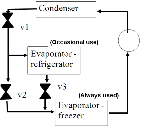
For example, one may wish to operate a freezer permanently but an additional chiller intermittently. With the chiller in use, the cycle is operated so that V1 causes refrigerant to expand to an intermediate pressure (saturation temp say \(4^oC\)) and V3 causes refrigerant to expand to a low pressure (sat. temp say \(-18^oC\)) and V2 is closed. Opening V2 causes refrigerant to bypass the first evaporator - the flow impedance of V2 is far less than that of V3.
Figure 10 A unit that always provides freezing and occasionally provides cooling
Absorption Refrigeration
This is a form of heat operated refrigeration. A conventional compressor is replaced with a heat driven device. This can be advantageous because fuel is generally far cheaper than electricity or mechanical power, indeed one trend is to use waste heat from diesel generators or solar heat and convert this to cooling in summer. Absorption chillers are far quieter than vapour compressor cycles, and can operate across a bigger range of cooling powers with good COP.
In effect, one replaces a source of mechanical power with a heat engine. From the second law (Kelvin statement) the engine must not only have heat added to it but must also reject heat, in addition to heat rejected by the condenser.
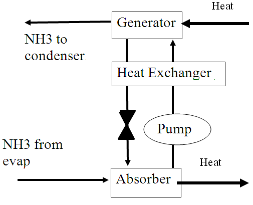
Let us consider the ammonia-water system - ammonia acts as the refrigerant. The diagram shows the right hand side of the system only - the compressor as it were - and the (omitted) left hand side comprises the usual condenser, throttle and evaporator. It is required that ammonia vapour exiting the evaporator is compressed before it enters the condenser. Ammonia is soluble in water at moderate temperature and is taken into solution in the absorber operating at typically 30 oC. Combining ammonia and water releases a heat of solution, rejected to the surroundings in conformity with the demands of the second law (see previous paragraph). The solution is pressurised by means of a pump, and one notes that the power of pumping as little asroughly of 0.2% of cooling power because solution is practically incompressible and pumping demands only work. We shall omit discussion of the heat exchanger for the time being. Ammonia vapour must be released from the solution at the higher, condenser pressure and this happens on heat addition, again in conformity with the generator.
Figure 11 The “compressor” part of an absorption chiller (water-ammonia)
The function of releasing high pressure vapour is achieved inside the generator operating at typically 90oC. The resulting solution is termed "weak" - it has a reduced concentration of NH3 - and is returned to the absorber. (Conversely the more concentrated solution exiting the absorber is termed "strong".)
Let us now return to consideration of the heat exchanger. We notice that weak solution (exiting generator) will require heating and strong solution (exiting absorber) will require cooling and there is a useful opportunity to recover heat. Stoeker and Jones give some worked examples for absorption chillers (H2O-LiBr, not H2O-NH3) and demonstrate that the heat exchanger increases COP from 71\% to 78\%.
Gas Cycles
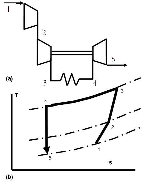
The refrigerant does not have to evaporate in order to effect cooling. When compressed air is available at ambient temperature, its expansion to 1 atm will reduce its temperature to well below the ambient value. This principle is often exploited to provide air conditioning in aircraft and is also exploited in cryogenic distillation (preparation of O2, N2 etc). An air cycle unit was demonstrated some years ago at the University's FRPERC Langford laboratory, now defunct. It operated as follows.
1-2-3 Two compressors act on the air. Air exits the second compressor at a high temperature.
3-4 By means of a heat exchanger, the compressed air is cooled to near ambient temperature.
4-5 The compressed air is expanded to 1 atm and cools. Work recovered from the turbine (4-5) is employed to drive the second compressor (2-3).
Mechanical power is supplied to the first compressor only (1-2).
Figure 12 Air Cycle Refrigeration
Variations on the above plant find use in aerospace applications.
The Peltier Effect
Until the 1990s this was employed mainly for controlling the cold references of thermal cameras. The cost of thermoelectric modules has reduced dramatically and the Peltier effect is now used in comparatively cheap units. For example computer gaming enthusiasts use them to cool central processing units. The coefficient of performance is very poor ( \(<40\%\) ).
Let us start with the Seebeck effect, a useful phenomenon which permits temperature measurement by means of thermocouples. At a junction between two dissimilar metals, an e.m.f. is generated in proportion to the thermodynamic temperature of the junction (in Kelvin). Joining a hot and cold junction creates a net e.m.f. in approximate proportion to the hot-to-cold temperature difference. Note that (classically) this is detected with a Galvanometer - a very sensitive voltmeter - and the junctions are arranged such that identical types of wire are connected at the galvanometer terminals.
The
causes of the Seebeck effect lie well outside the topic of Thermodynamics and the expertise of this lecturer; internet sources refer to charge-carrier diffusion, phonon drag and Thompson effect.
Peltier observed that the effect could be reversed. That is, when a current flows through two thermocouple junctions heat heat is rejected at one junction and absorbed at the other (as illustrated). The effect is minor when metal-to-metal junctions are employed, but semi-conductor devices are now freely available at low cost (about £40) allowing typically 10 watts of cooling.


 \begin{equation}
h_9 = x h_3 + (1-x)h_2 = 0.0745 \times 1445.5 + (1-0.0745) \times 1576 = 1576 - 0.0745 \times 182.2 = 1562 kJ/kg
\end{equation}
$$h_4 = 1680 kJ/kg $$
\begin{equation}
h_9 = x h_3 + (1-x)h_2 = 0.0745 \times 1445.5 + (1-0.0745) \times 1576 = 1576 - 0.0745 \times 182.2 = 1562 kJ/kg
\end{equation}
$$h_4 = 1680 kJ/kg $$