
These notes support an interactive web that predicts heat transfer rates . The bare essentials of the topic are introduced.
Some thermodynamicists might well restrict their interests to heat transfer through the cylinder walls of a Sterling Engine, heat transfer into boilers (either in power plant or historic railway locomotives), and heat transfer to the evaporation and condensation coils of heat pumps. More widely, engineers will tackle heat losses from buildings, heat losses from insulated piping and process vessels, cooling of electronic equipment, and a wide range of heat transfer problems in Chemical and Process Engineering. Heat transfer is a broad subject supported by extensive specialist literature; for many problems engineers must research and read literature carefully before attempting design problems. Nonetheless, for some sets of preliminary engineering estimates the simple methods presented here might produce estimates of heat flows with modest accuracty.
A typical problem would involve one or more layers of insulation, separating warm and cold fluid. It might or might not be necessary to use a heat transfer coefficient to estimate the thermal resistances of thermal boundary layers covering the left-hand and right hand surfaces of the insulation pack.
The screen dumps below show isometric views of slabs and temperature profiles.
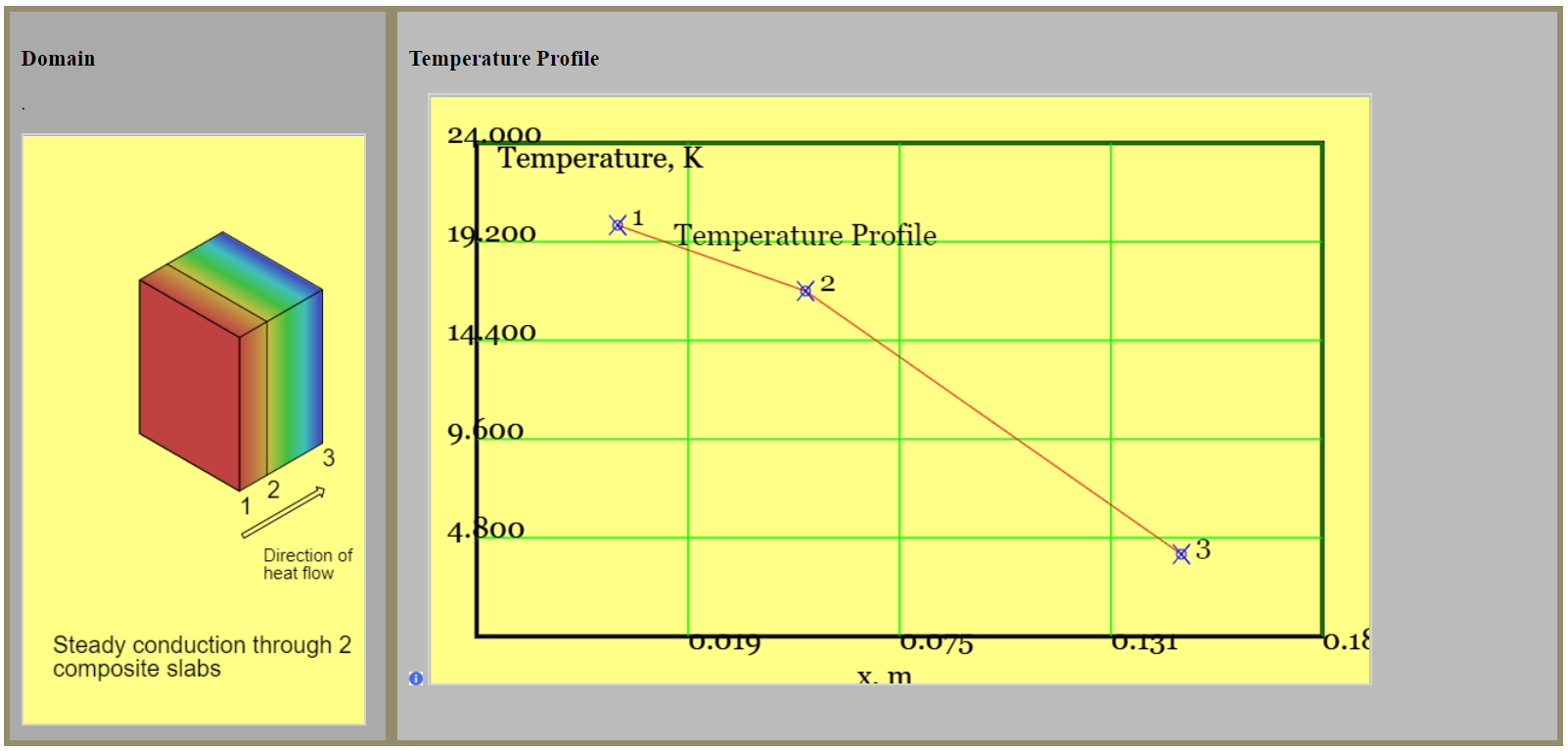
(a)
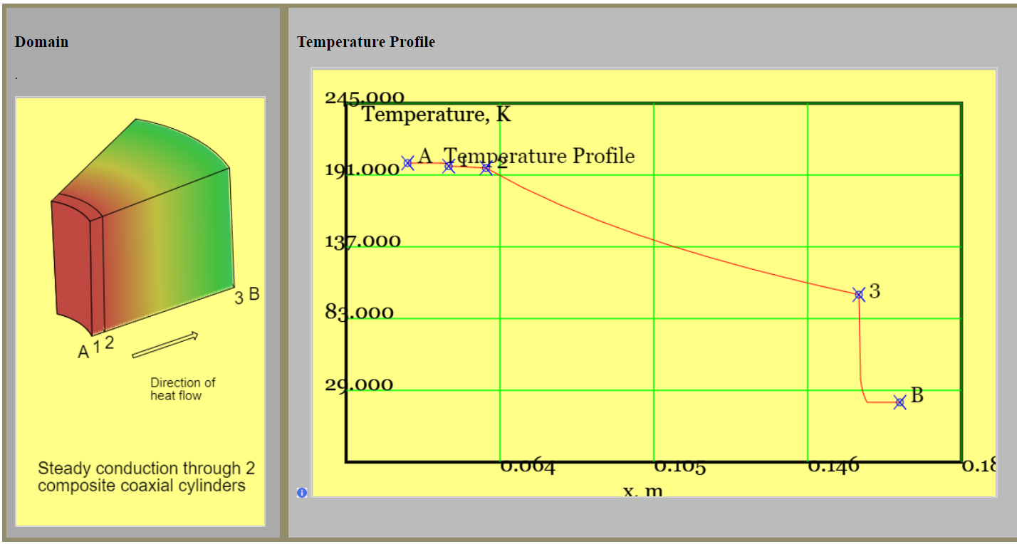
(b)
Figure 1: Geometric arrangements of slabs and temperature profiles: (a) two composite rectangular slabs with temperatures specified on the surfaces of face 1 (red) and face 3 (blue), (b) two composite annuli with temperatures specified in the free stream at positions A and B. Owing to the temperature loss through the boundary layer (3-B) face 3 is not coloured blue. Layer faces are numbered 1,2,3. Free streams are labelled A,B.
Heat transfer by thermal conduction is treated as moving in one direction only: the x-direction (rectangular slabs) or the r-direction (cylinders or spheres). In consequence, there is no heat loss through the flanks of the slab. The slabs are assumed to be at steady-state; the temperature profile with the slab is constant. In consequence, the heat addition to the slab is equal to the heat rejection: we concern ourselves with a single rate of heat flow. There is no internal heat generation (e.g. by radioactive decay). There is no moving boundary work.
A system's electrical resistance is the applied potential difference required to drive one unit of current flow. Its thermal resistance is the applied temperature difference required to drive one unit of heat flow rate.
From the Fourier-Biot Law of heat conduction, one derives a general expression for the rate of heat conduction through a solid prismatic section,
$$ \dot{Q} = -\lambda A \frac{ \Delta T }{\Delta x} $$where \( \dot{Q} \) is the rate of heat transfer , \( \lambda \) is a material constant termed the "thermal conductivity", \( A \) is an average cross-section area of the prism. Also \( \Delta T \ = T_2-T_1 \) is the difference in temperature between the two slab faces, and \( \Delta x \) is the slab thickness.
Let us propose a thermal resistance that is analogous to electrical resistance. Let the two ends of a current carrier (i.e. a resistor) be at electrical potential \( \phi_1 \) and \( \phi_2 \). The electrical resistance relates either to Ohm's Law, or the geometric and material properties of the resistor.
$$ R = \frac{\phi_1-\phi_2}{I} = \frac{-\Delta \phi}{I} = \frac{V}{I} = \frac{\Delta x}{A \sigma} \qquad electrical \; resistance $$where V is the decrease in potential (the "voltage") and \( \sigma \) is a material constant termed "electrical conductivity". The thermal analogue is, $$ R = \frac{T_1-T_2}{\dot{Q}} = \frac{-\Delta T}{\dot{Q}} = \frac{\Delta x}{A \lambda} \qquad thermal \; resistance $$
For a series of (for example) three electrical resistances the total electrical resistance is the sum of the component resistances. This conforms to the overall potential difference being the sum of the differences across the individual resistors.
$$ V_{ov} = \phi_1-\phi_4 = -1 \times ((\phi_4-\phi_3) + (\phi_3 - \phi_2) + (\phi_2 - \phi_1)) $$and the intermediate potentials, \( \phi_2 , \phi_3 \), cancel. Note that electrical current I is a constant throughout the circuit, and substitute Ohm's law, \( \phi_4-\phi_3 =-I R_{34} \) etc, for each potential difference on the far right hand side, and substitute Ohm's Law, \(V_{ov} = I R_{ov} \), for the voltage on the far left hand side.
$$ I R_{ov} = I (R_{12} + R_{23} + R_{34} ) \implies R_{ov} = R_{12} + R_{23} + R_{34} ... $$The thermal resistance is analagous; heat conduction rate is substituted for the constant current and temperature differences are substituted for potential differences (voltages). The thermal resistance of prismatic rectangular slab then becomes,
$$ R = \frac {-\Delta T }{\dot{Q}} = \frac{ \Delta x }{\lambda A} $$Cylindrical and spherical co-ordinate systems employ a principal r-direction rather than an x-direction, and one writes,
$$ \dot{Q} = -\lambda A_{av} \frac{ \Delta T }{\Delta r} \implies R = \frac{\Delta r}{ A_{av} \lambda } $$where \(A_{av}\) is an average cross sectional area. (Unlike the prism or rectangular slab, A is not constant and thus \( A_2 > A_1 \) ). For an annulus the logarithmic mean area applies.
$$ A_{av} = \frac{A_2-A_1}{ln(A_2/A_1)}= 2 \pi L \frac{r_2-r_1}{ln(r_2/r_2)} \implies \dot{Q}= -2 \pi L \lambda \frac{ \Delta T }{ln(r_2/r_1)} $$(The heat transfer rate on the far right hand side is frequently quoted in text books.) For spherical shells the geometric mean area applies.
$$ A_{av} = \sqrt{A_1 \times A_2} = 4 \pi r_1 r_2 \implies \dot{Q} = -\frac { 4 \pi r_1 r_2 \lambda \Delta T }{ r_2 - r_1} $$The exterior slab surfaces might well be heated or cooled by a fluid and, rather than the surface temperatures of solid layers, the problem might well specified in terms of the fluids' bulk or free stream temperatures. The topic of natural convection is extensive and complex (please see warning at the start of this note) and only some indicative ideas follow. In short, engineers consider a range of complex physical processes - natural convection, mixed convection, forced convection, boiling, condensation - and characterise their heat transmission by a single coefficient. This may (depending on physical process) assume that most (say 95 per cent) or resistance happens within a very thin boundary layer coating the solid surface. The heat transfer from the free stream to a solid surface is then approximated as
$$ \dot{Q} = \alpha A (T_s - T_w) $$where \( \alpha \) is the heat transfer coefficient, s indicates a free stream temperature (for external flows) or a bulk temperature (for internal flows), and w indicates a surface temperture. Do not confuse heat convection with heat conduction; the processes are very different. Do not confuse heat transfer coefficient with thermal conductivity; the constants are very different. Some indicative values of heat transfer coefficient are on the Engineering Toolbox website - you will see very wide ranges of estimates here. For more precise work, start be reading carefully a good text book such as Incropera and De Witt or Chapman . You will see that the heat transfer coefficient depends on many things - surface roughness, fluid material properties, velocity, geometrical arrangments of fluid passages, flow regime and (particularly for boiling and natural convection) the temperature difference.
The resistance of a thermal boundary layer could be written as,
$$ R_{conv} = \frac{1}{\alpha A} $$
The visualisation assoicated with this note estimates thermal resistances for each component in a series. The steady rate of heat flow through said series is then,
$$ \dot{Q} = -\frac{ \Delta T}{R_{ov}} $$If we allow for boundary layers the free stream temperatures are given subscripts A and B and for N layers the heat flow rate becomes,
$$ \dot{Q} = \frac{ T_A-T_B}{R_A + R_{12}+R_{23} ... + R_{N,N+1} + R_B} $$Whereas if tempertures are specified at external faces,
$$ \dot{Q} = \frac{ T_1-T_{N+1}}{ R_{12}+R_{23} ... + R_{N,N+1} } $$There are, unfortunately, some issues with reporting thermal resistances. They are not widely used in some branches of engineeering, and not widely reported in some text books; so much so that some authors seem to confuse "thermal resistance" with "thermal resistance for one unit area of cross section". A more widely reported concept is the overall heat transfer coefficient , or "U-value".
$$ \dot{Q} = U A_{ref} |\Delta T| = \frac {|\Delta T|}{R} $$One must take care in specifying the reference area - for the purposes of our web page we use the outer surface of the cylinder or sphere. (For rectangular slabs the area is constant.)
Consider a wall measuring 1metre x 3 metres in cross section. The wall comprises two sections: the first 5cm thick with a thermal conductivity of 0.2 W/mK, and the second 10cm thick with a thermal conductivity of 0.1 W/mK. The inner surface is 16K hotter than the outer surface. Estimate the heat loss through the wall
Solution: See Figure 1a. The heat flow is, $$ \dot{Q} = \frac {\lambda_{12} A}{x_2-x_1} (T_1-T_2) = \frac {\lambda_{23} A}{x_2-x_3} (T_3-T_2) $$
Identify the two thermal resistances (thickess divided by (conductivity-times-area)) and add to get total resistance
$$ \dot{Q} = \frac {T_1-T_3}{ \frac{x_2-x_1}{\lambda_{12} A} + \frac{x_3-x_2}{\lambda_{23} A} }$$ $$ \dot{Q} = \frac{16}{\frac{0.05}{0.2 \times 3} + \frac{0.1}{0.1 \times 3}} = \frac{16}{0.0833+0.333} = \frac{16}{0.4167} watts$$ $$ \dot{Q} = 38.4 watts $$The denominator terms correspond to resistances \(R_{12}\) and \( R_{23} \). If we treat the circuit in the same way as a potential divider, then we can (if required) obtain the intermediate temperature.
$$ T_2 = T_1 - (T_1-T_3) \frac{R_{12}}{R_{12}+ R_{23}} = T_1 - 16 \frac{8.33e-2}{8.33e-2+ 3.333e-1} = T_1-3.2K $$An insulated AISI-316 stainless steel pipe carries steam. Estimate the rate of heat loss per metre length of pipe. The inner diameter of the pipe is 10 cm, the pipe wall is 1cm-thick and has a thermal conductivity of 16.3 W/mK. The insulation is 10cm-thick and has a thermal conductivity of 1.2 W/mK. The heat transfer coefficients are \( 1000 W m^{-2} K^{-1} \) on the steam side and \( 9 W m^{-2} K^{-1} \) on the air side. The steam temperature is \(200^oC\) and the air temperature is \(20^oC\).
Solution: See Figure 1b. The heat flow is,
$$ \dot{Q}= 2 \pi r_1 L \alpha_A (T_A-T_1) + \frac{2 \pi L \lambda_{12}}{ln(r_2/r_1)} (T_1-T_2) + \frac{2 \pi L \lambda_{23}}{ ln(r_3/r_2)} (T_2-T_3) + 2 \pi r_3 L \alpha_B (T_3-T_B) $$Identify the four thermal resistances ( \( -\Delta T_{layer}/ \dot{Q} \) ) and add to get total resistance. Note the factor of \( 2 \pi L \),
$$ \dot{Q}= 2 \pi L \frac {T_A-T_B} {\frac{1}{r_1 \alpha_A} + \frac {ln(r_2/r_1)} { \lambda_{12}} + \frac { ln(r_3/r_2)} { \lambda_{23}} + \frac{1}{r_3 \alpha_B}} $$where \(r_1=0.05m, r_2=0.06m, r_3=0.016m\) are radii , and \( L=1.0m\) is the pipe length. (Do not forget that radius is half pipe diameter.)
$$ \dot{Q}= 2 \pi \times 1 \times \frac{200-20}{\frac{1}{0.05 \times 1000} + \frac{ln(6/5)}{16.3} + \frac{ln(16/6)}{1.2} + \frac{1}{0.016 \times 9 } } $$
$$ \dot{Q}= \frac{200-20}{3.18 \times 10^{-3} + 1.78 \times 10^{-3} + 0.1301 + 0.1105} = 733.0 watts $$It is useful to find the overall heat transfer coefficient, using the outermost area as a reference area,
$$ A_{ref} = 2 \pi r_3 L = 2 \pi \times 0.016 \times 1 = 1.005 m^2 $$ $$ U = \frac{\dot{Q}}{A_{ref} (T_A-T_B)} = \frac{733}{1.005 \times (200-20)} = 40.5 W m^{-2} K^{-1} $$